1. Bayesian Inference

Modern Bayesian statistics is mostly performed using computer code. This has dramatically changed how Bayesian statistics was performed from even a few decades ago. The complexity of models we can build has increased, and the barrier of necessary mathematical and computational skills has been lowered. Additionally, the iterative modeling process has become, in many aspects, much easier to perform and more relevant than ever. The popularization of very powerful computer methods is really great but also demands an increased level of responsibility. Even if expressing statistical methods is easier than ever, statistics is a field full of subtleties that do not magically disappear by using powerful computational methods. Therefore having a good background about theoretical aspects, especially those relevant in practice, is extremely useful to effectively apply statistical methods. In this first chapter, we introduce these concepts and methods, many of which will be further explored and expanded throughout the rest of the book.

1.1. Bayesian Modeling

A conceptual model is a representation of a system, made of the composition of concepts that are used to help people know, understand, or simulate the object or process the model represents [6]. Additionally, models are human-designed representations with very specific goals in mind. As such, it is generally more convenient to talk about the adequacy of the model to a given problem than its intrinsic correctness. Models exist solely as an aid to a further goal.

When designing a new car, a car company makes a physical model to help others understand how the product will look when it is built. In this case, a sculptor with prior knowledge of cars, and a good estimate of how the model will be used, takes a supply of raw material such as clay, uses hand tools to sculpt a physical model. This physical model can help inform others about various aspects of the design, such as whether the appearance is aesthetically pleasing, or if the shape of the car is aerodynamic. It takes a combination of domain expertise and sculpting expertise to achieve a useful result. The modeling process often requires building more than one model, either to explore different options or because the models are iteratively improved and expanded as a result of the interaction with other members of the car development team. These days it is also common that in addition to a physical car model, there is a digital model built-in Computer-Aided Design software. This computer model has some advantages over a physical one. It is simpler and cheaper to use for digital for crash simulations versus testing on physical cars. It is also easier to share this model with colleagues in different offices.

These same ideas are relevant in Bayesian modeling. Building a model requires a combination of domain expertise and statistical skill to incorporate knowledge into some computable objectives and determine the usefulness of the result. Data is the raw material, and statistical distributions are the main mathematical tools to shape the statistical model. It takes a combination of domain expertise and statistical expertise to achieve a useful result. Bayesian practitioners also build more than one model in an iterative fashion, the first of which is primarily useful for the practitioner themselves to identify gaps in their thinking, or shortcomings in their models. These first sets of models are then used to build subsequent improved and expanded models. Additionally, the use of one inference mechanism does not obviate the utility for all others, just as a physical model of a car does not obviate the utility of a digital model. In the same way, the modern Bayesian practitioner has many ways to express their ideas, generate results, and share the outputs, allowing a much wider distribution of positive outcomes for the practitioner and their peers.

1.1.1. Bayesian Models

Bayesian models, computational or otherwise, have two defining characteristics:

• Unknown quantities are described using probability distributions [1]. We call these quantities parameters [2].

• Bayes’ theorem is used to update the values of the parameters conditioned on the data. We can also see this process as a reallocation of probabilities.

At a high-level we can describe the process of constructing Bayesian modeling in 3 steps.

1. Given some data and some assumptions on how this data could have been generated, we design a model by combining and transforming random variables.

2. We use Bayes’ theorem to condition our models to the available data. We call this process inference, and as a result we obtain a posterior distribution. We hope the data reduces the uncertainty for possible parameter values, though this is not a guarantee of any Bayesian model.

3. We criticize the model by checking whether the model makes sense according to different criteria, including the data and our expertise on the domain-knowledge. Because we generally are uncertain about the models themselves, we sometimes compare several models.

If you are familiar with other forms of modeling, you will recognize the importance of criticizing models and the necessity of performing these 3 steps iteratively. For example, we may need to retrace our steps at any given point. Perhaps we introduced a, silly, coding mistake, or after some challenges we found a way to improve the model, or we find that the data is not useful as we originally thought, and we need to collect more data or even a different kind of data.

Throughout this book we will discuss different ways to perform each of these 3 steps and we will learn about ways to expand them into a more complex Bayesian workflow. We consider this topic so important that we dedicated an entire Chapter 9 to revisit and rediscuss these ideas.

1.1.2. Bayesian Inference

In colloquial terms, inference is associated with obtaining conclusions based on evidence and reasoning. Bayesian inference is a particular form of statistical inference based on combining probability distributions in order to obtain other probability distributions. Bayes’ theorem provides us with a general recipe to estimate the value of the parameter \(\boldsymbol{\theta}\) given that we have observed some data \(\boldsymbol{Y}\):

(1.1)\[\underbrace{p(\boldsymbol{\theta} \mid \boldsymbol{Y})}_{\text{posterior}} = \frac{\overbrace{p(\boldsymbol{Y} \mid \boldsymbol{\theta})}^{\text{likelihood}}\; \overbrace{p(\boldsymbol{\theta})}^{\text{prior}}}{\underbrace{{p(\boldsymbol{Y})}}_{\text{marginal likelihood}}}\]

The likelihood function links the observed data with the unknown parameters while the prior distribution represents the uncertainty [3] about the parameters before observing the data \(\boldsymbol{Y}\). By multiplying them we obtain the posterior distribution, that is the joint distribution over all the parameters in the model (conditioned on the observed data). Fig. 1.1 shows an example of an arbitrary prior, likelihood and the resulting posterior [4].

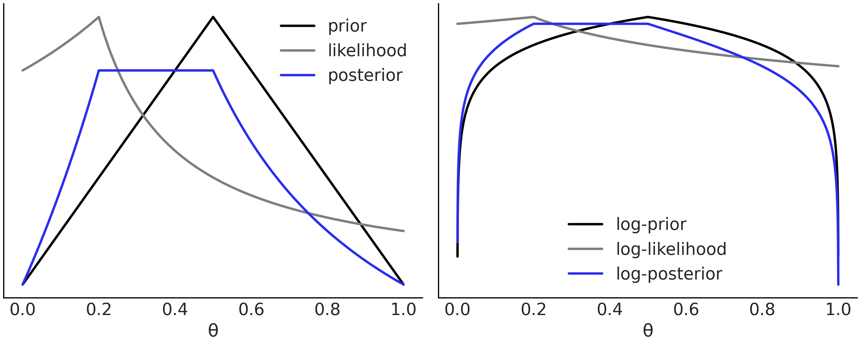
Fig. 1.1 Left panel. A hypothetical prior indicating that the value \(\theta = 0.5\) is more likely and the plausibility of the rest of the values decreases linearly and symmetrically (black). A likelihood showing that the value \(\theta = 0.2\) is the one that better agrees with the hypothetical data (gray) and the resulting posterior (blue), a compromise between prior and likelihood. We have omitted the values of the y-axis to emphasize that we only care about relative values. Right panel, the same functions as in the left panel but the y-axis is in the log-scale. Notice that the information about relative values is preserved, for example, the location of the maxima and minima is the same in both panels. The log scale is preferred to perform calculations as computations are numerically more stable.

Notice that while \(\boldsymbol{Y}\) is the observed data, it also is a random vector as its values depend on the results of a particular experiment [5]. In order to obtain a posterior distribution, we regard the data as fixed at the actual observed values. For this reason a common alternative notation is to use \(y_{obs}\), instead of \(\boldsymbol{Y}\).

As you can see evaluating the posterior at each specific point is conceptually simple, we just need to multiply a prior times a likelihood. However, that is not enough to inform us about the posterior, as we not only need the posterior probability at that specific point, but also in relation to the surrounding points. This global information of the posterior distribution is represented by the normalizing constant. Unfortunately, difficulties arise from the need to compute the normalizing constant \(p(\boldsymbol{Y})\). This is easier to see if we write the marginal likelihood as:

(1.2)\[{p(\boldsymbol{Y}) = \int_{\boldsymbol{\Theta}} p(\boldsymbol{Y} \mid \boldsymbol{\theta})p(\boldsymbol{\theta}) d\boldsymbol{\theta}}\]

where \(\Theta\) means we are integrating over all the possible values of \(\theta\).

Computing integrals like this can be much harder than would first appear (see Section Marginal Likelihood and a funny XKCD comic [6]). Especially when we realize that for most problems a closed-form expression is not even available. Fortunately, there are numerical methods that can help us with this challenge if used properly. As the marginal likelihood is not generally computed, it is very common to see Bayes’ theorem expressed as a proportionality:

(1.3)\[\underbrace{p(\boldsymbol{\theta} \mid \boldsymbol{Y})}_{\text{posterior}} \propto \overbrace{p(\boldsymbol{Y} \mid \boldsymbol{\theta})}^{\text{likelihood}}\; \overbrace{p(\boldsymbol{\theta})}^{\text{prior}}\]

A note on notation

In this book we use the same notation \(p(\cdot)\) to represent different quantities, like a likelihood function and a prior probability distribution. This is a slightly abuse of notation but one we find useful. This notation provides the same epistemological status to all quantities. Additionally it reflects that even when the likelihood is not strictly a probability density function, we just do not care as we only think about the likelihood in the context of a prior and vice versa. In other words, we think of both quantities as equally necessary elements of models in order to compute a posterior distribution.

One nice feature of Bayesian statistics is that the posterior is (always) a distribution. This fact allows us to make probabilistic statements about the parameters, like the probability of a parameter \(\boldsymbol{\tau}\) being positive is 0.35. Or the most likely value of \(\boldsymbol{\phi}\) is 12 with a 50% chance of being between 10 and 15. Moreover, we can think of the posterior distribution as the logical consequence of combining a model with the data, and thus the probabilistic statements derived from them are guaranteed to be mathematically consistent. We just need to remember that all these nice mathematical properties are only valid in the platonic world of ideas where mathematical objects such as spheres, Gaussians and Markov chains exist. As we move from mathematical purity into the applied math messiness of the real world we must always keep in mind that our results are conditioned not only on the data but also on the models. Consequently, bad data and/or bad models could lead to nonsensical statements, even if they are mathematically consistent. We must always have a healthy quota of skepticism about our data, models, and results. To make this more explicit, we may want to express Bayes’ theorem in a more nuanced way:

(1.4)\[p(\boldsymbol{\theta} \mid \boldsymbol{Y}, M) \propto p(\boldsymbol{Y} \mid \boldsymbol{\theta}, M) \; p(\boldsymbol{\theta}, M)\]

Emphasizing that our inferences are always dependent on the assumptions made by model \(M\).

Having said that, once we have a posterior distribution we can use it to derive other quantities of interest. This is generally done by computing expectations, for example:

(1.5)\[J = \int f(\boldsymbol{\theta}) \; p(\boldsymbol{\theta} \mid \boldsymbol{Y}) \; d\boldsymbol{\theta}\]

If \(f\) is the identity function \(J\) will turn out be the mean [7] of \(\boldsymbol{\theta}.\):

(1.6)\[\bar{\boldsymbol{\theta}} = \int_{\boldsymbol{\Theta}} \boldsymbol{\theta} p(\boldsymbol{\theta} \mid \boldsymbol{Y}) d\boldsymbol{\theta}\]

The posterior distribution is the central object in Bayesian statistics, but it is not the only one. Besides making inferences about parameter values, we may want to make inferences about data. This can be done by computing the prior predictive distribution:

(1.7)\[p(\boldsymbol{Y}^\ast) = \int_{\boldsymbol{\Theta}} p(\boldsymbol{Y^\ast} \mid \boldsymbol{\theta}) \; p(\boldsymbol{\theta}) \; d\boldsymbol{\theta}\]

This is the expected distribution of the data according to the model (prior and likelihood). That is the data we expect, given the model, before actually seeing any observed data \(\boldsymbol{Y}^\ast\). Notice that Equations (1.2) (marginal likelihood) and Equation (1.7) (prior predictive distribution) look really similar. The difference is in the former case, we are conditioning on our observed data \(Y\) while in the latter, we are not conditioning on the observed data. As a result the marginal likelihood is a number and the prior predictive distribution is a probability distribution.

We can use samples from the prior predictive distribution as a way to evaluate and calibrate our models using domain-knowledge. For example, we may ask questions such as “Is it OK for a model of human heights to predict that a human is -1.5 meters tall?”. Even before measuring a single person, we can recognize the absurdness of this query. Later in the book we will see many concrete examples of model evaluation using prior predictive distributions in practice, and how the prior predictive distributions inform the validity, or lack thereof, in subsequent modeling choices.

Bayesian models as generative models

Adopting a probabilistic perspective for modeling leads to the mantra models generate data [4]. We consider this concept to be of central importance. Once you internalize it, all statistical models become much more clear, even non-Bayesian ones. This mantra can help to create new models; if models generate data, we can create suitable models for our data just by thinking of how the data could have been generated! Additionally, this mantra is not just an abstract concept. We can adopt a concrete representation in the form of the prior predictive distribution. If we revisit the 3 steps of Bayesian modeling, we can re-frame them as, write a prior predictive distribution, add data to constrain it, check if the result makes sense. Iterate if necessary.

Another useful quantity to compute is the posterior predictive distribution:

(1.8)\[p(\tilde{\boldsymbol{Y}} \mid \boldsymbol{Y}) = \int_{\boldsymbol{\Theta}} p(\tilde{\boldsymbol{Y}} \mid \boldsymbol{\theta}) \, p(\boldsymbol{\theta} \mid \boldsymbol{Y}) \, d\boldsymbol{\theta}\]

This is the distribution of expected, future, data \(\tilde{\boldsymbol{Y}}\) according to the posterior \(p(\boldsymbol{\theta} \mid \boldsymbol{Y})\), which in turn is a consequence of the model (prior and likelihood) and observed data. In more common terms, this is the data the model is expecting to see after seeing the dataset \(\boldsymbol{Y}\), i.e. these are the model’s predictions. From Equation (1.8), we can see that predictions are computed by integrating out (or marginalizing) over the posterior distribution of parameters. As a consequence predictions computed this way will incorporate the uncertainty about our estimates.

Bayesian posteriors in a Frequentist light

Because posteriors are derived from the model and the observed data only, we are not making statements based on non-observed, but potentially observed realizations of the underlying data-generating process. Inferring on non-observed is generally done by the so called frequentists methods. Nevertheless, if we use posterior predictive samples to check our models we are (partially) embracing the frequentist idea of thinking about non-observed but potentially observable data. We are not only comfortable with this idea, we will see many examples of this procedure in this book. We think it is one honking great idea — let us do more of these!

1.2. A DIY Sampler, Do Not Try This at Home

Closed form expressions for the integral in Equation (1.2) are not always possible and thus much of modern Bayesian inference is done using numerical methods that we call Universal Inference Engines (see Section Inference Methods) just to compensate for the fact we live in the \(21^\text{st}\) century and we still do not have flying cars. Anyway, there are many well-tested Python libraries providing such numerical methods so in general it is very unlikely that a Bayesian practitioner will need to code their own Universal Inference Engine.

As of today there are generally only two good reasons to code your own engine, you are either designing a new engine that improves on the old ones, or you are learning how the current engines work. Since we are learning in this chapter we will code one, but for the rest of the book we are going to use engines available in Python libraries.

There are many algorithms that can be used as Universal Inference Engines. Probably the most widely adopted and powerful is the family of Markov chain Monte Carlo methods (MCMC). At a very high level, all MCMC methods approximate the posterior distribution using samples. The samples from the posterior distribution are generated by accepting or rejecting samples from a different distribution called the proposal distribution. By following certain rules [8] and under certain assumptions, we have theoretical guarantees that we will get samples that are a good approximation of the posterior distribution. Thus, MCMC methods are also known as samplers. All these methods require to be able to evaluate the prior and likelihood at a given parameter value. That is, even when we do not know what the entire posterior looks like, we can ask for its density point-wise.

One such algorithm is Metropolis-Hastings [7, 8, 9]. This is not a very modern or particularly efficient algorithm, but Metropolis-Hastings is simple to understand and also provides a foundation to understand more sophisticated and powerful methods. [9]

The Metropolis-Hasting algorithm is defined as follows:

1. Initialize the value of the parameter \(\boldsymbol{X}\) at \(x_i\)

2. Use a proposal distribution [10] \(q(x_{i + 1} \mid x_i)\) to generate a new value \(x_{i + 1}\) from the old one \(x_i\).

3. Compute the probability of accepting the new value as:

   (1.9)\[p_a (x_{i + 1} \mid x_i) = \min \left (1, \frac{p(x_{i + 1}) \; q(x_i \mid x_{i + 1})} {p(x_i) \; q (x_{i + 1} \mid x_i)} \right)\]

4. If \(p_a > R\) where \(R \sim \mathcal{U}(0, 1)\), save the new value, otherwise save the old one.

5. Iterate 2 to 4 until a sufficiently large sample of values has been generated

The Metropolis algorithm is very general and can be used in non-Bayesian applications but for what we care in this book, \(p(x_i)\) is the posterior’s density evaluated at the parameter value \(x_i\). Notice that if \(q\) is a symmetric distribution the terms \(q(x_i \mid x_{i + 1})\) and \(q(x_{i + 1} \mid x_i)\) will cancel out (conceptually it means it is equally likely are we are to go from \(x_{i+1}\) to \(x_i\) or to go from \(x_{i}\) to \(x_{i+1}\)), leaving just the ratio of the posterior evaluated at two points. From Equation (1.9) we can see this algorithm will always accept moving from a low probability region to a higher one and will probabilistically accept moving from a high to low probability region.

Another important remark is that the Metropolis-Hastings algorithm is not an optimization method! We do not care about finding the parameter value with the maximum probability, we want to explore the \(p\) distribution (the posterior). This can be seen if we take note that once at a maximum, the method can still move to a region of lower probabilities in subsequent steps.

To make things more concrete let us try to solve the Beta-Binomial model. This is probably the most common example in Bayesian statistics and it is used to model binary, mutually-exclusive outcomes such as 0 or 1, positive or negative, head or tails, spam or ham, hotdog or not hotdog, healthy or unhealthy, etc. More often than not Beta-Binomial model is used as the first example to introduce the basics of Bayesian statistics, because it is a simple model that we can solve and compute with ease. In statistical notation we can write the Beta-Binomial models as:

(1.10)\[ \begin{align}\begin{aligned}\begin{split}\begin{split} \theta \sim &\; \text{Beta}(\alpha, \beta) \\ Y \sim &\; \text{Bin}(n=1, p=\theta)\end{split}\\\end{split}\end{aligned}\end{align} \]

In Equation (1.10) we are saying the parameter \(\theta\) has \(\text{Beta}(\alpha, \beta)\) as its prior distribution. And we assume the data is distributed following a Binomial distribution \(\text{Bin}(n=1, p=\theta)\), which represents our likelihood distribution. In this model the number of successes \(\theta\) can represent quantities like the proportion of heads or the proportion of dying patients, sometimes statistics can be a very dark place. This model has an analytical solution (see Conjugate Priors) for the details. For the sake of the example, let us assume we do not know how to compute the posterior, and thus we will implement the Metropolis-Hastings algorithm into Python code in order to get an approximate answer. We will do it with the help of SciPy statistical functions:

Listing 1.1 metropolis_hastings_sampler

def post(θ, Y, α=1, β=1):
    if 0 <= θ <= 1:
        prior = stats.beta(α, β).pdf(θ)
        like  = stats.bernoulli(θ).pmf(Y).prod()
        prob = like * prior
    else:
        prob = -np.inf
    return prob

We also need data, so we will generate some random fake data for this purpose.

Listing 1.2 metropolis_hastings_sampler_rvs

Y = stats.bernoulli(0.7).rvs(20)

And finally we run our implementation of the Metropolis-Hastings algorithm:

Listing 1.3 metropolis_hastings

n_iters = 1000
can_sd = 0.05
α = β =  1
θ = 0.5
trace = {"θ":np.zeros(n_iters)}
p2 = post(θ, Y, α, β)

for iter in range(n_iters):
    θ_can = stats.norm(θ, can_sd).rvs(1)
    p1 = post(θ_can, Y, α, β)
    pa = p1 / p2

    if pa > stats.uniform(0, 1).rvs(1):
        θ = θ_can
        p2 = p1

    trace["θ"][iter] = θ

At line 9 of Code Block metropolis_hastings we generate a proposal distribution by sampling from a Normal distribution with standard deviation can_sd. At line 10 we evaluate the posterior at the new generated value θ_can and at line 11 we compute the probability of acceptance. At line 17 we save a value of θ in the trace array. Whether this value is a new one or we repeat the previous one, it will depend on the result of the comparison at line 13.

Ambiguous MCMC jargon

When we use Markov chain Monte Carlo Methods to do Bayesian inference, we typically refer to them as MCMC samplers. At each iteration we draw a random sample from the sampler, so naturally we refer to the output from MCMC as samples or draws. Some people make the distinction that a sample is made up by a collection of draws, others treat samples and draws as interchangeably.

Since MCMC draws samples sequentially we also say we get a chain of draws as result, or just MCMC chain for short. Usually it is desired to draw many chains for computational and diagnostic reasons (we discuss how to do this in Chapter 2). All the output chains, whether singular or plural, are typically referred to as a trace or simply the posterior. Unfortunately spoken language is imprecise so if precision is needed the best approach is to review the code to understand exactly what is happening.

Note that the code implemented in Code Block metropolis_hastings is not intended to be efficient, in fact there are many changes that would be present in production-grade code, like computing the probabilities on the log scale to avoid under/overflow issues (see Section Log Probabilities), or pre-computing the proposal and the Uniform values. This is where the purity of math needs to be adjusted to meet the reality of computers, and why building these engines is best left to experts. Similarly, the value of can_sd, is a parameter of the Metropolis-Hastings algorithm, not a parameter from the Bayesian model. In theory this parameter should not affect the correct behavior of the algorithm, but in practice it is very important as the efficiency of the method will certainly be affected by its value (see Section Inference Methods for an in-depth discussion).

Returning to our example, now that we have our MCMC samples we want to understand what it looks like. A common way to inspect the results of a Bayesian inference is to plot the sampled values per iteration together with a histogram, or other visual tool, to represent distributions. For example, we can use the code in Code Block diy_trace_plot to plot Fig. 1.2 [11]:

Listing 1.4 diy_trace_plot

_, axes = plt.subplots(1,2, sharey=True)
axes[0].plot(trace['θ'], '0.5')
axes[0].set_ylabel('θ', rotation=0, labelpad=15)
axes[1].hist(trace['θ'], color='0.5', orientation="horizontal", density=True)
axes[1].set_xticks([])

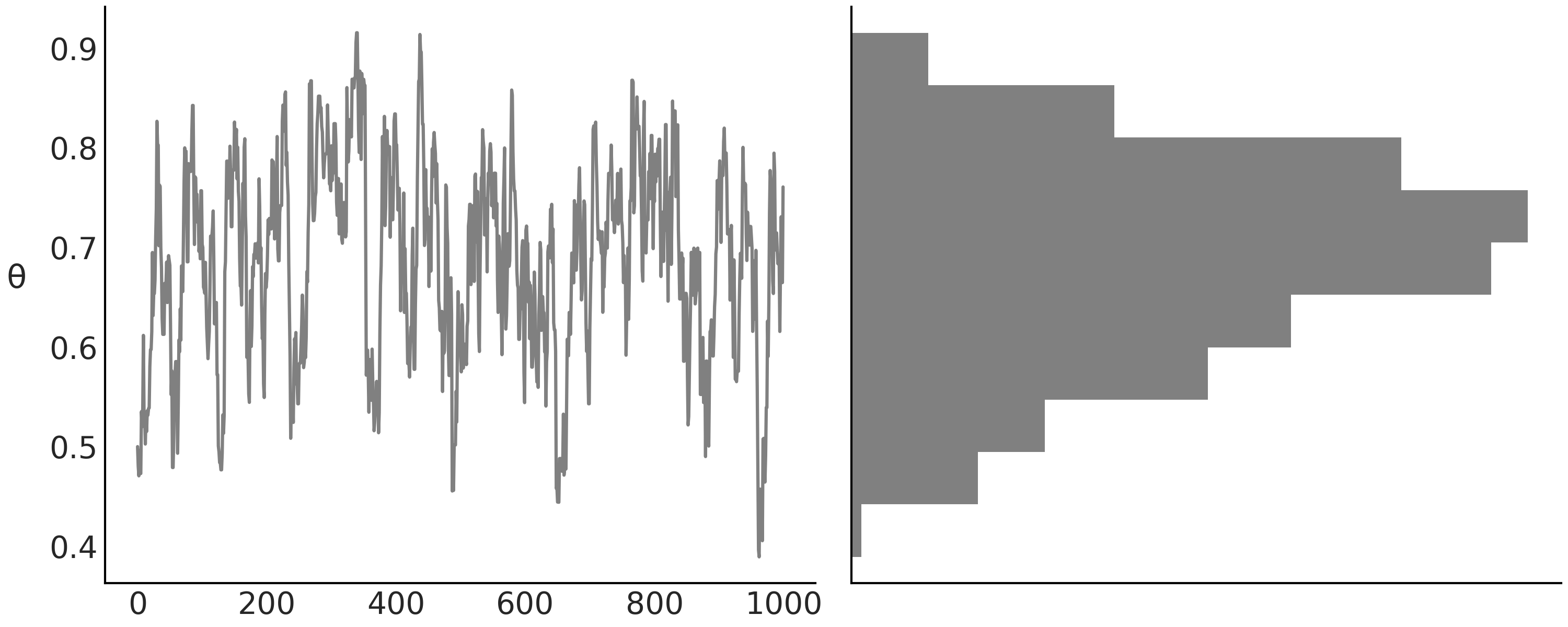
Fig. 1.2 On the left, we have the sampled values of the parameter \(\theta\) at each iteration. On the right, we have the histogram of the sampled values of \(\theta\). The histogram is rotated, to make it easier to see that both plots are closely related. The plot on the left shows the sequence of sampled values. This sequence is our Markov Chain. The plot on the right shows the distribution of the sampled values.

Generally it is also useful to compute some numerical summaries. Here we will use the Python package ArviZ [3] to compute these statistics:

az.summary(trace, kind="stats", round_to=2)

Table 1.1 Posterior summary

	mean	sd	hdi_3%	hdi_97%
\(\theta\)	0.69	0.01	0.52	0.87

ArviZ’s function summary computes the mean, standard deviation and the highest density interval (HDI) 94% of our parameter \(\theta\). The HDI is the shortest interval containing a given probability density, 94% for this particular example [12]. Fig. 1.3, generated with az.plot_posterior(trace) is a close visual equivalent of the above summary in Table 1.1. We can see the mean and the HDI, on top of a curve representing the entire posterior distribution. The curve is computed using a kernel density estimator (KDE), which is like the smooth version of a histogram. ArviZ uses KDEs in many of its plots, and even internally for a few computations.

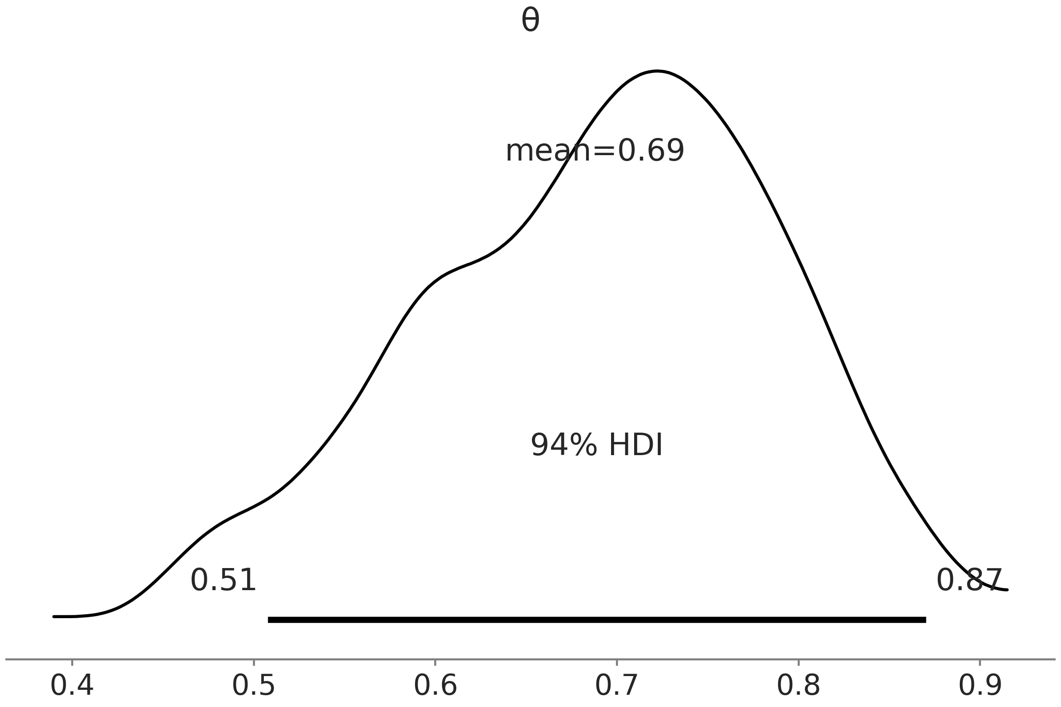
Fig. 1.3 Posterior plot visualizing the samples generated from Code Block metropolis_hastings. The posterior distribution is represented using a KDE, the mean and the limits of the HDI 94% are represented in the figure.

The HDI is a common choice in Bayesian statistics and round values like 50% or 95% are commonplace. But ArviZ uses 94% (or 0.94) as the default value as seen in both the summary Table 1.1 and Fig. 1.3. The reason for this choice is that 94 is close to the widely used 95 but is different enough to serve as a friendly reminder that there is nothing special about these round values [10]. Ideally you should choose a value that fits your needs [11], or at least acknowledge that you are using a default.

1.3. Say Yes to Automating Inference, Say No to Automated Model Building

Instead of writing our own sampler and having to define our models using scipy.stats method we can leverage the aid of Probabilistic Programming Languages (PPL). These tools allow users to express Bayesian models using code and then perform Bayesian inference in a fairly automated fashion thanks to Universal Inference Engines. In short PPLs help practitioners focus more on model building and less on the mathematical and computational details. The availability of such tools has helped increase the popularity and usefulness of Bayesian methods in the last few decades. Unfortunately, these Universal Inference Engines methods are not really that universal, as they will not be able to efficiently solve every Bayesian model (but we still like the cool name!). Part of the job of the modern Bayesian practitioner is being able to understand and work around these limitations.

In this book we will use PyMC3 [1] and TensorFlow Probability [2]. Let us write the model from Equation (1.10) using PyMC3:

Listing 1.5 beta_binom

# Declare a model in PyMC3
with pm.Model() as model:
    # Specify the prior distribution of unknown parameter
    θ = pm.Beta("θ", alpha=1, beta=1)

    # Specify the likelihood distribution and condition on the observed data
    y_obs = pm.Binomial("y_obs", n=1, p=θ, observed=Y)

    # Sample from the posterior distribution
    idata = pm.sample(1000, return_inferencedata=True)

You should check by yourself that this piece of code provides essentially the same answer as our DIY sampler we used before, but with much less effort. If you are not familiar with the syntax of PyMC3, just focus on the intent of each line as shown in the code comments for now. Since we have defined our model in PyMC3 syntax we can also utilize pm.model_to_graphviz(model) to generate a graphical representation of the model in Code Block beta_binom (see Fig. 1.4).

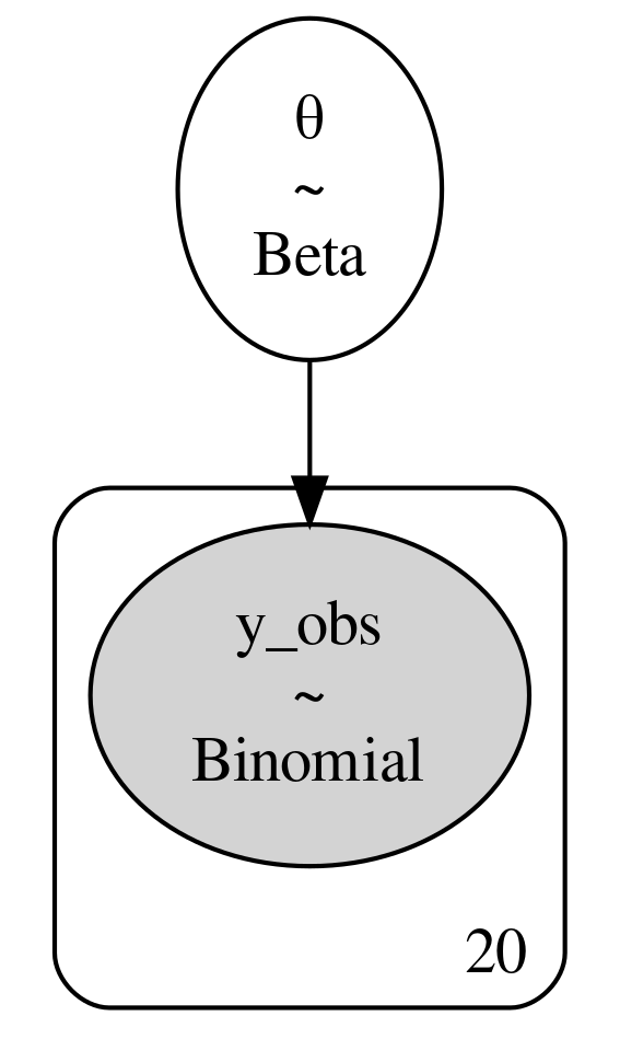
Fig. 1.4 A graphical representation of the model defined in Equation (1.10) and Code Block beta_binom. The ovals represent our prior and likelihood, whereas the 20 in this case indicates the number of observations. [fig:BetaBinomModelGraphViz]{#fig:BetaBinomModelGraphViz label=”fig:BetaBinomModelGraphViz”}

A Probabilistic Programming Language can not only evaluate the log-probability of the random variables to get the posterior distribution, but also simulate from various distributions as well. For example, Code Block predictive_distributions shows how to use PyMC3 to generate 1000 samples from the prior predictive distribution and 1000 samples from the posterior predictive distribution. Notice how for the first one, we have a function taking the model as argument while for the second function we have to pass both model and trace, reflecting the fact that the prior predictive distribution can be computed just from the model while the posterior predictive distribution we need a model and posterior. The generated samples from the prior and posterior predictive distributions are represented in the top and bottom panel, respectively, from Fig. 1.5.

Listing 1.6 predictive_distributions

pred_dists = (pm.sample_prior_predictive(1000, model)["y_obs"],
              pm.sample_posterior_predictive(idata, 1000, model)["y_obs"])

Equations (1.1), (1.7), and (1.8) clearly define the posterior, the prior predictive, and the posterior predictive distributions as different mathematical objects. The two later are distributions over data and the first one is a distribution over the parameters in a model. Fig. 1.5 helps us visualize this difference and also includes the prior distribution for completeness.

Expressing models in multiple ways

There are numerous methods to communicate the architecture of statistical models. These can be, in no particular order:

• Spoken and written language

• Conceptual diagrams: Fig. 1.4.

• Mathematical notation: Equation (1.10)

• Computer Code: Code Block beta_binom

For a modern Bayesian practitioner it is useful to be literate across all these mediums. They are formats you see presented in talks, scientific papers, hand sketches when discussing with colleagues, code examples on the internet, etc. With fluency across these mediums you will be better able to understand concepts presented one way, and then apply them in another way. For example, read paper and then implement a model, or hear about a technique in a talk and then be able to write a blog post on it. For you personally fluency will likely speed up your learning and increase your ability to communicate with others. Ultimately this helps achieve what general statistics community always strives for a better shared understanding of the world.

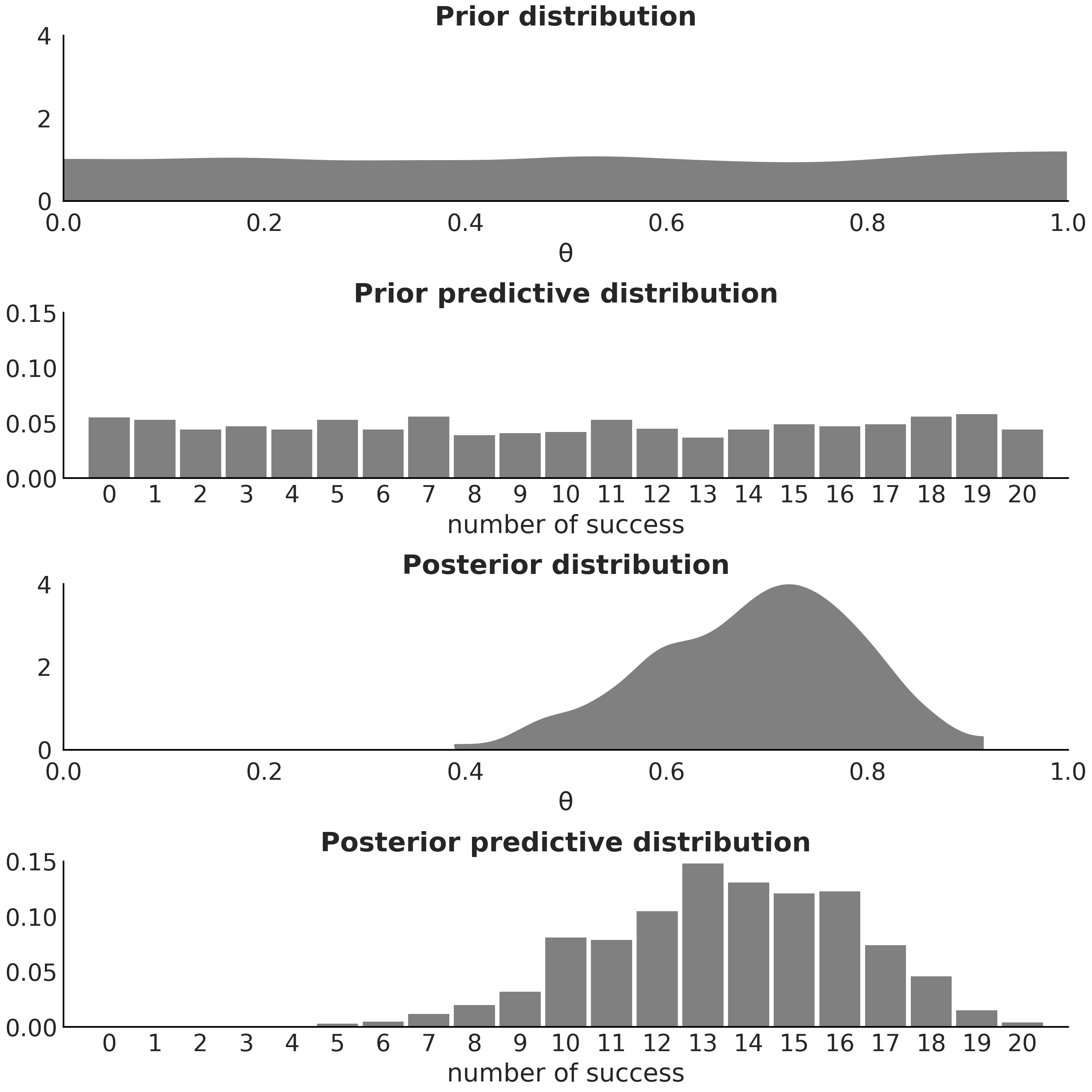
Fig. 1.5 From top plot to bottom plot we show: (1) samples from the prior distribution of the parameter \(\theta\); (2) samples from the prior predictive distribution, where we are plotting the probability distribution of the total number of successes; (3) posterior samples of the parameter \(\theta\); (4) posterior predictive distribution of the total number of successes. The x-axis and y-axis scales are shared between the first and third plots and then between the second and fourth plots.

As we already mentioned, posterior predictive distributions take into account the uncertainty about our estimates. Fig. 1.6 shows that the predictions using the mean are less spread than predictions from the posterior predictive distribution. This result is not only valid for the mean, we would get a similar picture if we change the mean to any other point-estimate.

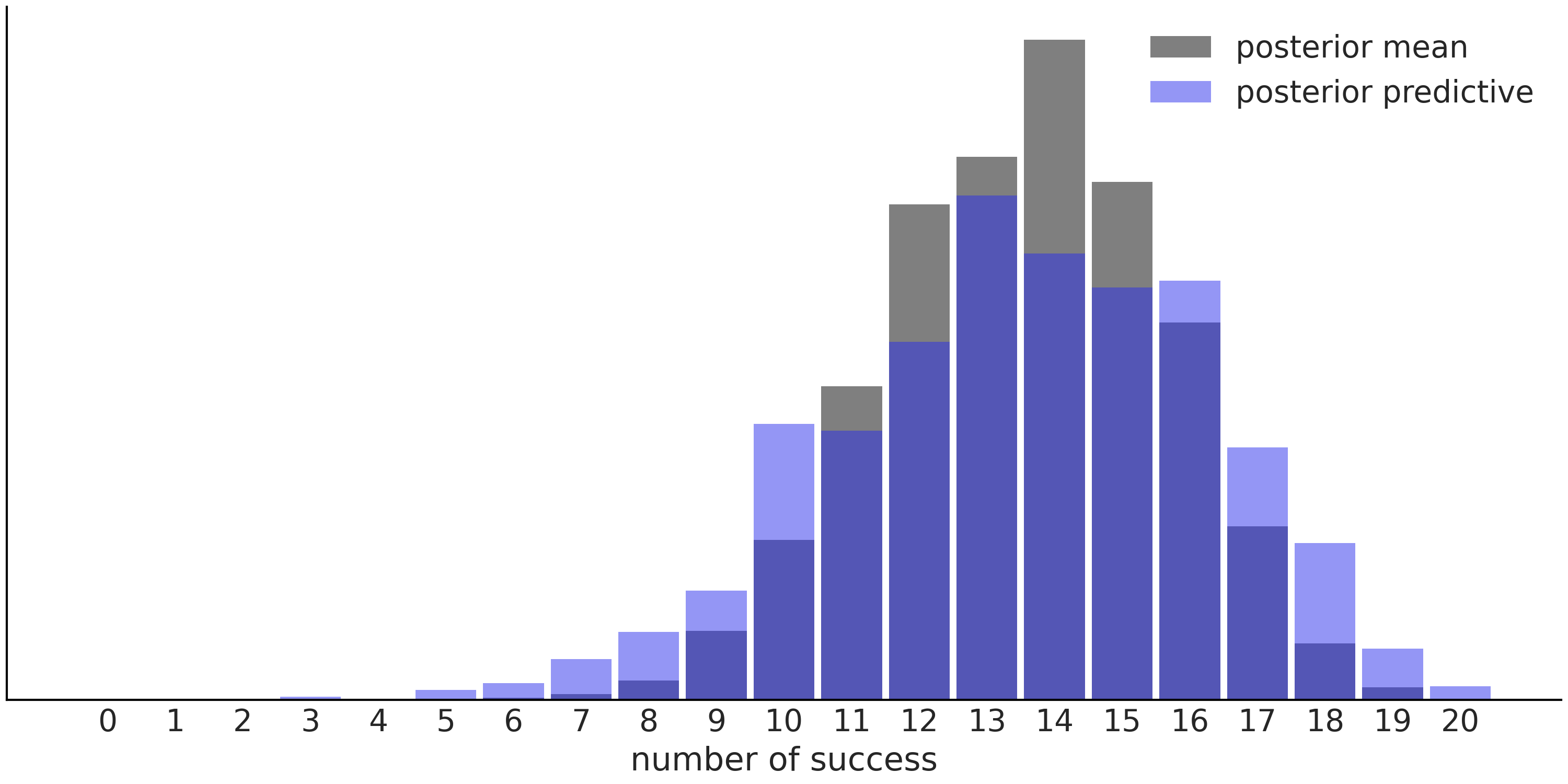
Fig. 1.6 Predictions for the Beta-Binomial model, using the posterior mean (gray histogram) vs predictions using the entire posterior, i.e. the posterior predictive distribution (blue histogram).

1.4. A Few Options to Quantify Your Prior Information

Having to choose a prior distribution is portrayed both as a burden and as a blessing. We choose to affirm that is a necessity, if you are not choosing your priors someone else is doing it for you. Letting others decide for you is not always a bad thing. Many of these non-Bayesian methods can be very useful and efficient if applied in the correct context, and with awareness of their limitations. However, we firmly believe there is an advantage for the practitioner in knowing the model assumptions and have the flexibility to alter them. Priors are just one form of assumption.

We also understand that prior elicitation can be a source of doubts, anxiety, and even frustration for many practitioners, especially for, but not necessarily only for, newcomers. Asking what is the best-ever prior for a given problem, is a common and totally valid question. But it is difficult to give a straight satisfying answer other than, there is no such thing. At best there are some useful defaults that we can use as starting points in an iterative modeling workflow.

In this section we discuss a few general approaches for selecting prior distributions. This discussion follows more or less an informativeness gradient from “blank slates” which include no information, to highly informative, which put as much information as possible into the priors. As with the other sections in this chapter, this discussion is more on the theoretical side. In the following chapters we will discuss how to choose priors in more practical settings.

1.4.1. Conjugate Priors

A prior is conjugate to a likelihood if the posterior belongs to the same family of distributions as the prior. For example, if the likelihood is Poisson and the prior Gamma, then the posterior will also be a Gamma distribution [13].

From a purely mathematical perspective, conjugate priors are the most convenient choice as they allow us to calculate the posterior distribution analytically with “pen and paper”, no complex computation required [14]. From a modern computational perspective, conjugate priors are generally not better than alternatives, the main reason being that modern computational methods allow us to perform inference with virtually any choice of priors and not just those that are mathematically convenient. Nevertheless, conjugate priors can be useful when learning Bayesian inference and also under some situations when there is a need to use analytical expressions for the posterior (see Section Example: Near Real Time Inference for an example). As is such, we will briefly discuss analytical priors using the Beta Binomial model.

As the name suggests, the conjugate prior for the binomial distribution is the Beta distribution:

(1.11)\[p(\theta \mid Y) \propto \overbrace{\frac{N!}{y!(N-y)!} \theta^y (1 - \theta)^{N-y}}^{\text{binomial-likelihood}} \: \overbrace{\frac{\Gamma(\alpha+\beta)}{\Gamma(\alpha)\Gamma(\beta)}\, \theta^{\alpha-1}(1-\theta)^{\beta-1}}^{\text{beta.prior}}\]

Because all the terms not depending on \(\theta\) are constant we can drop them and we get:

(1.12)\[p(\theta \mid Y) \propto \overbrace{\theta^y (1 - \theta)^{N-y}}^{\text{binomial-likelihood}} \: \overbrace{ \theta^{\alpha-1}(1-\theta)^{\beta-1}}^{\text{beta.prior}}\]

Reordering:

(1.13)\[p(\theta \mid Y) \propto \theta^{\alpha-1+y}(1-\theta)^{\beta-1+N-y}\]

If we want to ensure that the posterior is a proper probability distribution function, we need to add a normalization constant ensuring that the integral of the PDF is 1 (see Section Continuous Random Variables and Distributions). Notice that expression (1.13) looks like the kernel of a Beta distribution, thus by adding the normalization constant of a Beta distribution we arrive to the conclusion that the posterior distribution for a Beta-Binomial model is:

(1.14)\[p(\theta \mid Y) \propto \frac{\Gamma(\alpha_{post}+\beta_{post})}{\Gamma(\alpha_{post})\Gamma(\beta_{post})} \theta^{\alpha_{post}-1}(1-\theta)^{\beta_{post}-1} = \text{Beta}(\alpha_{post}, \beta_{post})\]

where \(\alpha_{post} = \alpha+y\) and \(\beta_{post} = \beta+N-y\).

As the posterior of a Beta-Binomial model is a Beta distribution we can use a Beta-posterior as the prior for a future analysis. This means that we will get the same result if we update the prior one data-point at a time or if we use the entire dataset at once. For example, the first four panels of Fig. 1.7 show how different priors get updated as we move from 0 to 1, 2, and 3 trials. The result is the same if we follow this succession or if we jump from 0 to 3 trials (or, in fact, \(n\) trials).

There are a lot of other interesting things to see from Fig. 1.7. For instance, as the number of trials increases, the width of the posterior gets lower and lower, i.e. the uncertainty gets lower and lower. Panels 3 and 5 show the results for 2 trials with 1 success and 12 trials with 6 success, for these cases, the sampling proportion estimator \(\hat \theta = \frac{y}{n}\) (black dot) is the same 0.5 for both cases (the posterior mode is also 0.5), although the width of the posteriors are concentrated in panel 5 reflecting that the number of observations is larger and thus uncertainty lower. Finally, we can see how different priors converge to the same posterior distribution as the number of observations increase. In the limit of infinite data, the posteriors (irrespective of priors used to compute those posteriors) will have all its density at \(\hat \theta = \frac{y}{n}\).

Listing 1.7 binomial_update

_, axes = plt.subplots(2,3, sharey=True, sharex=True)
axes = np.ravel(axes)

n_trials = [0, 1, 2, 3, 12, 180]
success = [0, 1, 1, 1, 6, 59]
data = zip(n_trials, success)

beta_params = [(0.5, 0.5), (1, 1), (10, 10)]
θ = np.linspace(0, 1, 1500)
for idx, (N, y) in enumerate(data):
    s_n = ("s" if (N > 1) else "")
    for jdx, (a_prior, b_prior) in enumerate(beta_params):
        p_theta_given_y = stats.beta.pdf(θ, a_prior + y, b_prior + N - y)

        axes[idx].plot(θ, p_theta_given_y, lw=4, color=viridish[jdx])
        axes[idx].set_yticks([])
        axes[idx].set_ylim(0, 12)
        axes[idx].plot(np.divide(y, N), 0, color="k", marker="o", ms=12)
        axes[idx].set_title(f"{N:4d} trial{s_n} {y:4d} success")

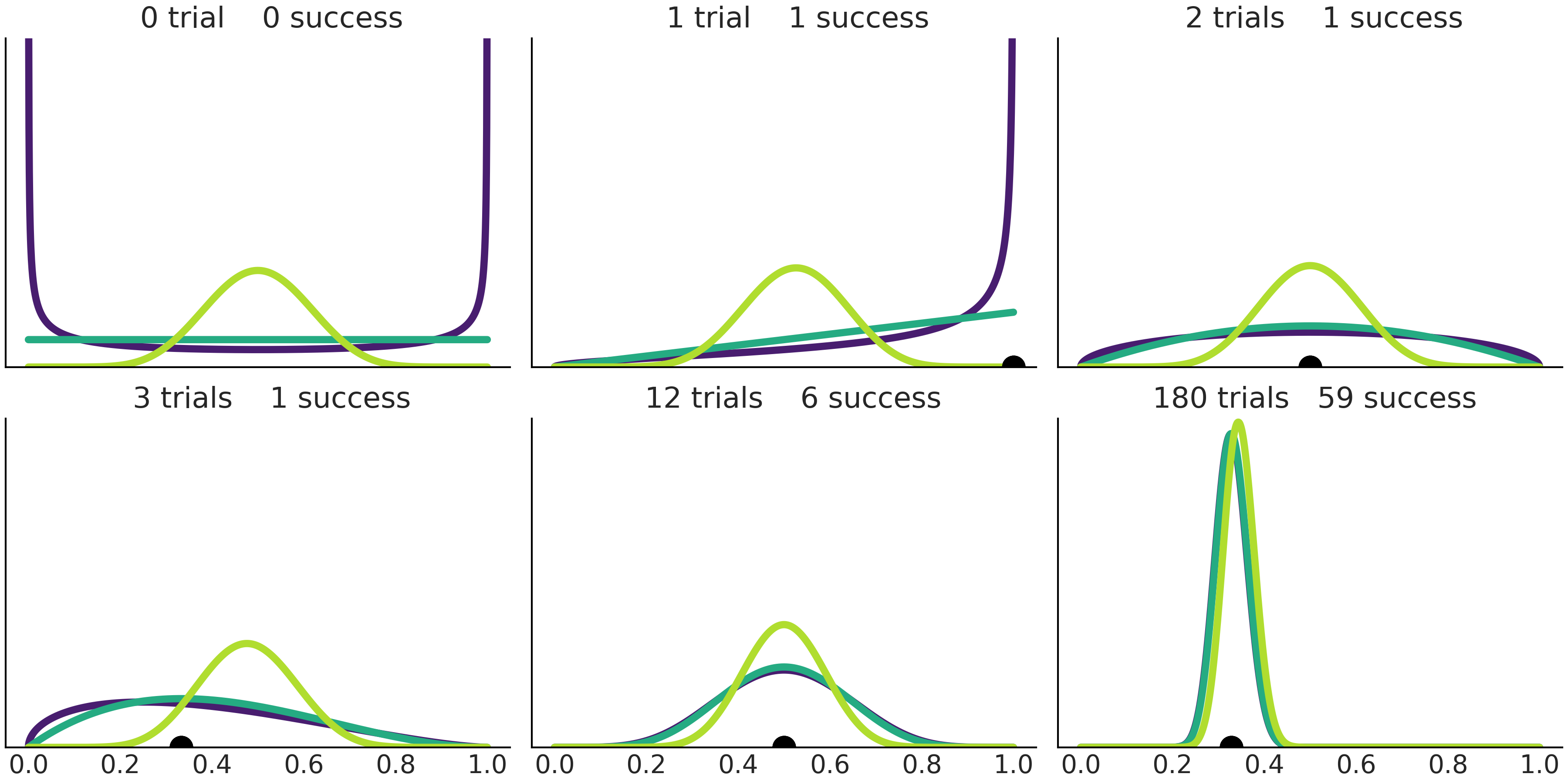
Fig. 1.7 Successive prior updating starting from 3 different priors and increasing the number of trials (and possible the number of successes too). The black dot represents the sampling proportion estimator \(\hat \theta = \frac{y}{n}\).

The mean of the Beta distribution is \(\frac{\alpha}{\alpha + \beta}\), thus the prior mean is:

(1.15)\[\mathbb{E}[\theta] = \frac{\alpha}{\alpha + \beta}\]

and the posterior mean is:

(1.16)\[\mathbb{E}[\theta \mid Y] = \frac{\alpha + y}{\alpha + \beta + n}\]

We can see that if the value of \(n\) is small in relation with the values of \(\alpha\) and \(\beta\) then the posterior mean will be closer to the prior mean. That is, the prior contributes more to the result than the data. If we have the opposite situation the posterior mean will be closer to the sampling proportion estimator \(\hat \theta = \frac{y}{n}\), in fact in the limit of \(n \rightarrow \infty\) the posterior mean will exactly match the sample proportion no matter which prior values we choose for \(\alpha\) and \(\beta\).

For the Beta Binomial model the posterior mode is:

(1.17)\[\operatorname*{argmax}_{\theta}{[\theta \mid Y]} = \frac{\alpha + y - 1}{\alpha + \beta + n - 2}\]

We can see that when the prior is Beta\((\alpha\!=\!1, \beta\!=\!1)\) (Uniform) the posterior mode is numerically equivalent to the sampling proportion estimator \(\hat \theta = \frac{y}{n}\). The posterior mode is often called the maximum a posteriori (MAP) value. This result is not exclusive for the Beta-Binomial model. In fact the results from many non-Bayesian methods can be understood as the MAP from Bayesian methods under some particular priors [15].

Compare Equation (1.16) to the sampling proportion \(\frac{y}{n}\). The Bayesian estimator is adding \(\alpha\) to the number of successes and \(\alpha + \beta\) to the number of trials. Which makes \(\beta\) the number of failures. In this sense we can think of the prior parameters as pseudo counts or if you want prior data. A prior \(\text{Beta}(1, 1)\) is equivalent to having two trials with 1 success and 1 failure. Conceptually, the shape of the Beta distribution is controlled by parameter \(\alpha\) and \(\beta\), the observed data updates the prior so that it shifts the shape of the Beta distribution closer and more narrowly to the majority of observations. For values of \(\alpha < 1\) and/or \(\beta < 1\) the prior interpretations becomes a little bit weird as a literal interpretation would say that the prior \(\text{Beta}(0.5, 0.5)\) corresponds to 1 trial with half failure and half success or maybe one trial with undetermined outcome. Spooky!

1.4.2. Objective Priors

In the absence of prior information, it sounds reasonable to follow the principle of indifference also known as the principle of insufficient reason. This principle basically says that if you do not have information about a problem then you do not have any reason to believe one outcome is more likely than any other. In the context of Bayesian statistics this principle has motivated the study and use of objective priors. These are systematic ways of generating priors that have the least possible influence on a given analysis. The champions of ascetic statistics favor objective priors as these priors eliminate the subjectivity from prior elicitation. Of course this does not remove other sources of subjectivity such as the choice of the likelihood, the data selection process, the choice of the problem being modeled or investigated, and a long et cetera.

One procedure to obtain objective priors is known as Jeffreys’ prior (JP). These type of priors are often referred as non-informative even when priors are always informative in some way. A better description is to say that JPs have the property of being invariant under reparametrization, i.e. writing an expression in a different but mathematically equivalent way. Let us explain what this exactly means with an example. Suppose Alice has a binomial likelihood with unknown parameter \(\theta\), she chooses a prior and computes a posterior. Alice’s friend Bob is interested on the same problem but instead of the number of success \(\theta\), Bob is interested on the odds of the success, i.e. \(\kappa\), with \(\kappa = \frac{\theta}{1-\theta}\). Bob has two choices: uses Alice’s posterior over \(\theta\) to compute \(\kappa\) [16] or choose a prior over \(\kappa\) to compute the posterior by himself. JPs guarantee that if both Alice and Bob use JPs then no matter which of the two choices Bob takes in order to compute the posteriors, he will get the same result. In this sense we say the results are invariant to the chosen parameterization. A corollary of this explanation could be, that unless we use JPs there is no guarantee that two (or more) parameterization of a model will necessarily lead to posteriors that are coherent.

For the one-dimensional case JP for \(\theta\) is

(1.18)\[p(\theta) \propto \sqrt{I(\theta)}\]

where \(I(\theta)\) is the expected Fisher information:

(1.19)\[I(\theta) = - \mathbb{E_{Y}}\left[\frac{d^2}{d\theta^2} \log p(Y \mid \theta)\right]\]

Once the likelihood function \(p(Y \mid \theta)\) has been decided by the practitioner, then the JP gets automatically determined, eliminating any discussion over prior choices, until that annoying person at the back of the conference room objects your choice of a JP in the first place.

For a detailed derivation of the JPs for both Alice and Bob problem see Section Jeffreys’ Prior Derivation. If you want to skip those details here we have the JP for Alice:

(1.20)\[p(\theta) \propto \theta^{-0.5} (1-\theta)^{-0.5}\]

This turns to be the kernel of the \(\text{Beta}(0.5, 0.5)\) distribution. Which is a u-shaped distribution as shown in the left-top panel of Fig. 1.8.

For Bob the JP is:

(1.21)\[p(\kappa) \propto \kappa^{-0.5} (1 + \kappa)^{-1}\]

This is a half-u-shaped distribution, defined in the \([0, \infty)\) interval, see top-right panel in Fig. 1.8. Saying this is a half-u-shaped may sound a little bit weird. Actually it is not that weird when we find that this is the kernel of a close cousin of the Beta distribution, the Beta-prime distribution with parameters \(\alpha=\beta=0.5\).

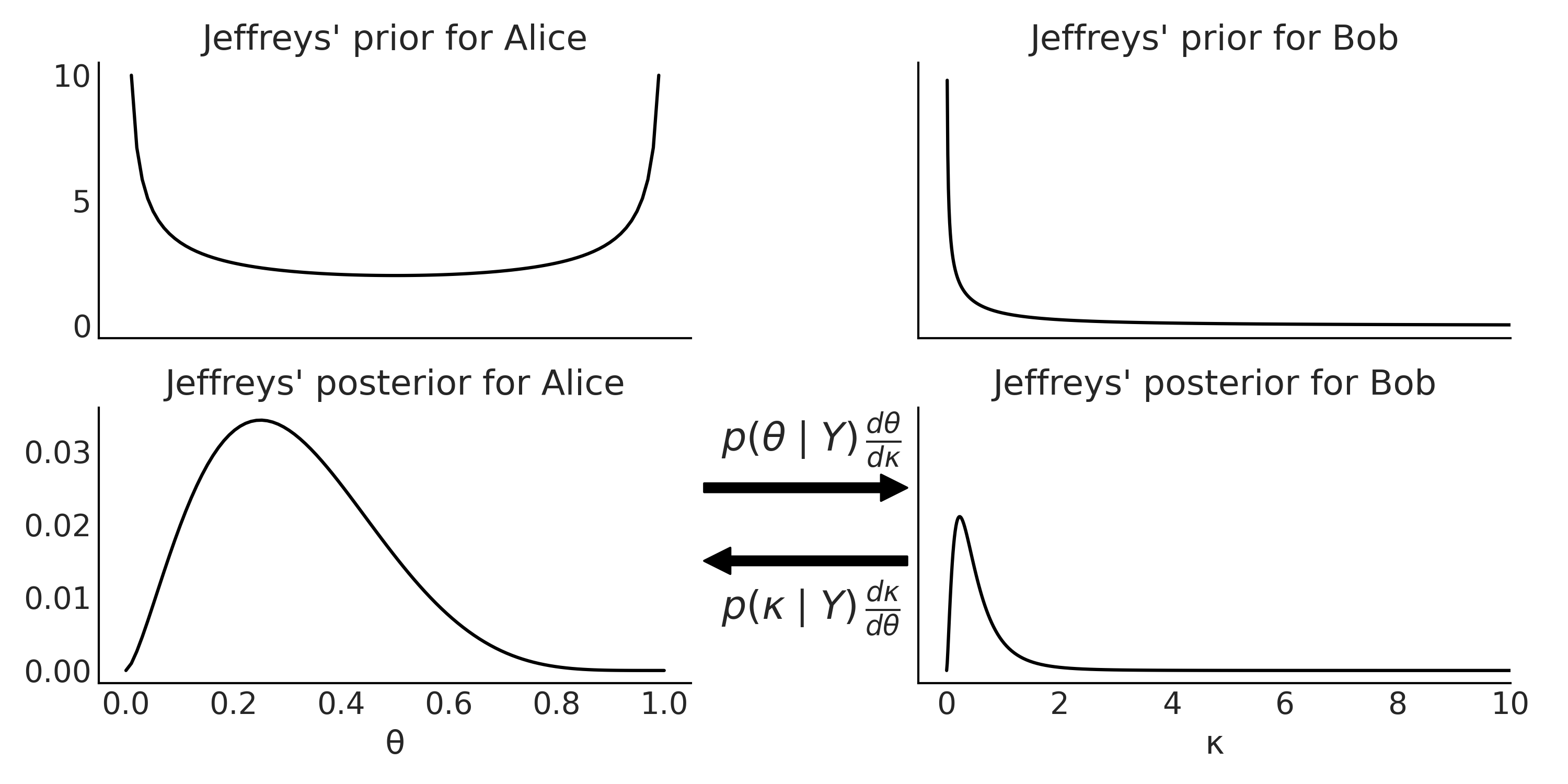
Fig. 1.8 Top: Jeffreys’ prior (unnormalized) for the binomial likelihood parameterized in term of the number of success \(\theta\) (left) or in term of the odds \(\kappa\) (right). Bottom: Jeffreys’ posteriors (unnormalized) for the binomial likelihood parameterized in term of the number of success \(\theta\) (left) or in term of the odds \(\kappa\) (right). The arrows between the posteriors indicate that the posterior are inter-convertible by applying the change of variable rule (see Section Transformations for details).

Notice that as the expectation in Equation (1.19) is with respect to \(Y \mid \theta\), that is an expectation over the sample space. This means that in order to obtain a JP we need to average over all possible experimental outcomes. This is a violation of the likelihood principle [17] as the inferences about \(\theta\) depends not just on the data at hand, but also on the set of potentially (but not yet) observed data.

A JP can be improper prior, meaning that it does not integrate to 1. For example, the JP for the mean of a Gaussian distribution of known variance is uniform over the entire real line. Improper priors are fine as long as we verify that the combination of them with a likelihood produces a proper posterior distribution, that is one integrating to 1. Also notice that we can not draw random samples from improper priors (i.e., they are non-generative) this can invalidate many useful tools that allow us to reason about our model.

JPs are not the only way to obtain an objective prior. Another possible route is to obtain a prior by maximizing the expected Kullback-Leibler divergence (see Section Kullback-Leibler Divergence) between the prior and posterior. These kind of priors are known as Bernardo reference priors. They are objective as these are the priors that allow the data to bring the maximal amount of information into the posterior distribution. Bernardo reference priors and Jeffreys’ prior do not necessarily agree. Additionally, objective priors may not exist or be difficult to derive for complicated models.

1.4.3. Maximum Entropy Priors

Yet another way to justify a choice of priors is to pick the prior with the highest entropy. If we are totally indifferent about the plausible values then such prior turns out to be the Uniform distribution over the range on plausible values [18]. But what about when we are not completely indifferent about the plausible values a parameter can take? For example, we may know our parameter is restricted to the \([0, \infty)\) interval. Can we obtain a prior that has maximum entropy while also satisfying a given constraint? Yes we can and that is exactly the idea behind maximum entropy priors. In the literature it is common to find the word MaxEnt when people talk about the maximum entropy principle.

In order to obtain a maximum entropy prior we need to solve an optimization problem taking into account a set of constraints. Mathematically this can be done using what is known as Lagrangian multipliers. Instead of a formal proof we are going to use a couple code examples to gain some intuition.

Fig. 1.9 shows 3 distributions obtained by entropy maximization. The purple distribution is obtained under no constraint, and we are happy to find that this is indeed the Uniform distribution as expected from the discussion about entropy in Section Entropy. If we do not know anything about the problem all events are equally likely a priori. The second distribution, in cyan, is obtained under the constraint that we know the mean value of the distribution. In this example the mean value is 1.5). Under this constraint we get an Exponential-like distribution. The last one in yellow-green was obtained under the restriction that the value 3 and 4 are known to appear with a probability of 0.8. If you check Code Block max_ent_priors you will see all distributions were computed under two constraints that probabilities can only take values in the interval \([0, 1]\) and that the total probability must be 1. As these are general constraints for valid probability distribution we can think of them as intrinsic or even ontological constraints. For that reason we say that the purple distribution in Fig. 1.9 was obtained under no-constraint.

Listing 1.8 max_ent_priors

cons = [[{"type": "eq", "fun": lambda x: np.sum(x) - 1}],
        [{"type": "eq", "fun": lambda x: np.sum(x) - 1},
         {"type": "eq", "fun": lambda x: 1.5 - np.sum(x * np.arange(1, 7))}],
        [{"type": "eq", "fun": lambda x: np.sum(x) - 1},
         {"type": "eq", "fun": lambda x: np.sum(x[[2, 3]]) - 0.8}]]

max_ent = []
for i, c in enumerate(cons):
    val = minimize(lambda x: -entropy(x), x0=[1/6]*6, bounds=[(0., 1.)] * 6,
                   constraints=c)['x']
    max_ent.append(entropy(val))
    plt.plot(np.arange(1, 7), val, 'o--', color=viridish[i], lw=2.5)
plt.xlabel("$t$")
plt.ylabel("$p(t)$")

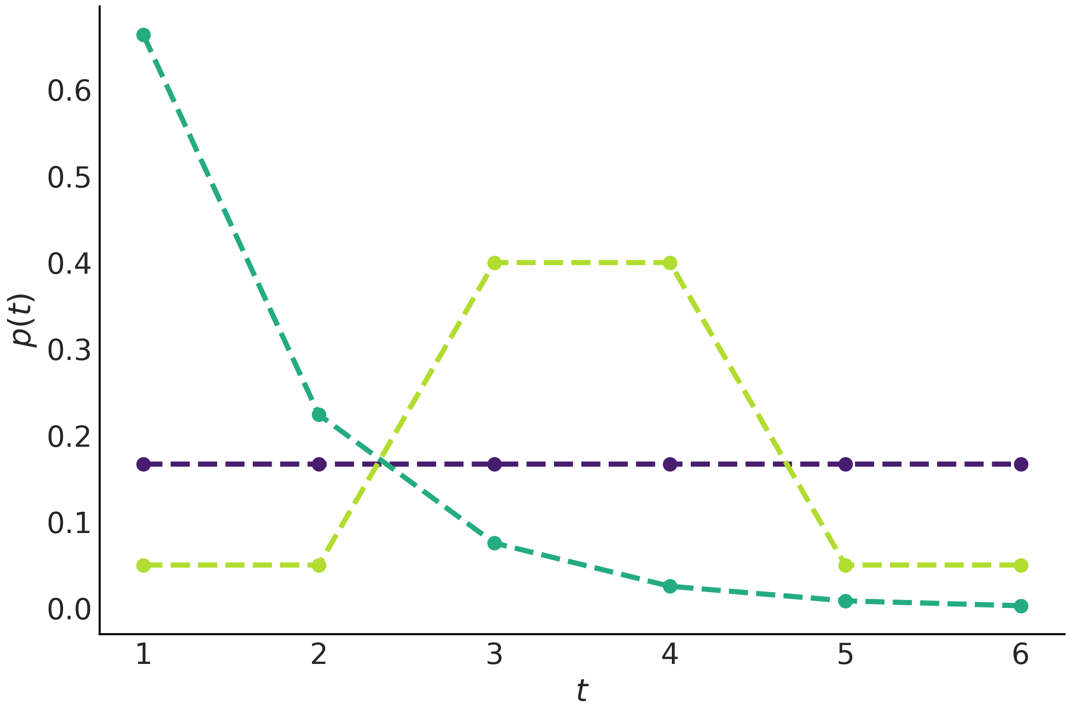
Fig. 1.9 Discrete distributions obtained by maximizing the entropy under different constraints. We are using the function entropy from scipy.stats to estimate these distributions. Notice how adding constraints can drastically change the distribution.

We can think of the maximum entropy principle as the procedure of choosing the flattest distribution, and by extension the flattest prior distribution, under a given constraint. In Fig. 1.9 the Uniform distribution is the flattest distribution, but notice that the distribution in green is also the flattest distribution once we include the restriction that the values 3 and 4 have a 80% chance of arising. Notice how the values 3 and 4 have both a probability of 0.4, even when you have infinite other ways to combine their probabilities to obtain the target value of 0.8, like 0+0.8, 0.7+0.1, 0.312+0.488 and so on. Also notice something similar is true for the values 1, 2, 5 and 6, they have a total probability of 0.2 which is evenly distributed (0.05 for each value). Now take a look at the Exponential-like curve, which certainly does not look very flat, but once again notice that other choices will be less flat and more concentrated, for example, obtaining 1 and 2 with 50% chance each (and thus zero change for the values 3 to 6), which will also have 1.5 as the expected value.

ite = 100_000
entropies = np.zeros((3, ite))
for idx in range(ite):
    rnds = np.zeros(6)
    total = 0
    x_ = np.random.choice(np.arange(1, 7), size=6, replace=False)
    for i in x_[:-1]:
        rnd = np.random.uniform(0, 1-total)
        rnds[i-1] = rnd
        total = rnds.sum()
    rnds[-1] = 1 - rnds[:-1].sum()
    H = entropy(rnds)
    entropies[0, idx] = H
    if abs(1.5 - np.sum(rnds * x_)) < 0.01:
        entropies[1, idx] = H
    prob_34 = sum(rnds[np.argwhere((x_ == 3) | (x_ == 4)).ravel()])
    if abs(0.8 - prob_34) < 0.01:
        entropies[2, idx] = H

Fig. 1.10 shows the distribution of entropies computed for randomly generated samples under the exact same conditions as the 3 distributions in Fig. 1.9. The dotted vertical line represents the entropy of the curves in Fig. 1.10. While this is not a proof, this experiment seems to suggest that there is no distribution with higher entropy than the distributions in Fig. 1.10, which is in total agreement with what the theory tells us.

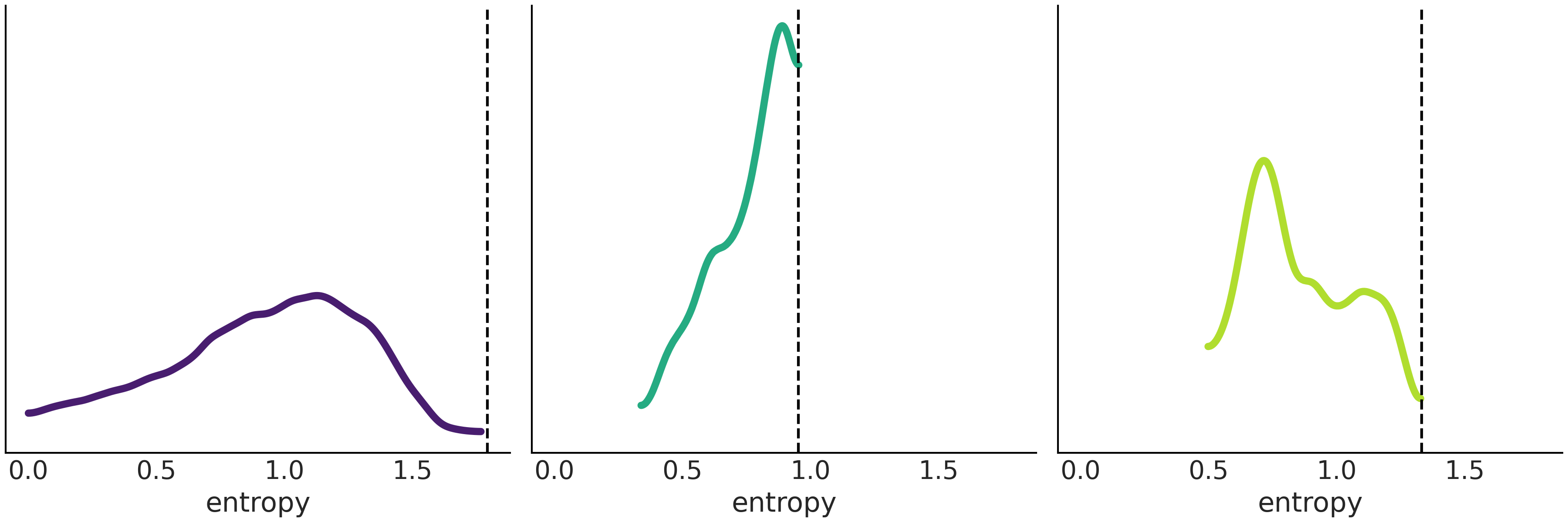
Fig. 1.10 The distribution of entropy for a set of randomly generated distributions. The dotted vertical line indicates the value for the distributions with maximum entropy, computed with Code Block max_ent_priors. We can see that none of the randomly generated distributions have an entropy larger that the distributions with maximum entropy, while this is no formal proof, this is certainly reassuring.

The distributions with the largest entropy under the following constraints are [19]:

• No constraints: Uniform (continuous or discrete, according to the type of variable)

• A positive mean, with support \([0, \infty)\): Exponential

• An absolute deviation to the mean, with support \((-\infty, \infty)\): Laplace (also known as double Exponential)

• A given mean and variance, with support \((-\infty, \infty)\): Normal distribution

• A given mean and variance, with support \([-\pi, \pi]\): Von Mises

• Only two unordered outcomes and a constant mean: Binomial, or the Poisson if we have rare events (the Poisson can be seen as a special case of the binomial)

It is interesting to note that many of the generalized linear models like the ones described in Chapter 3 are traditionally defined using maximum entropy distributions, given the constraints of the models. Similar to objective priors, MaxEnt prior may not exist or are difficult to derive.

1.4.4. Weakly Informative Priors and Regularization Priors

In previous sections we used general procedures to generate vague, non-informative priors designed to not put too much information into our analysis. These procedures to generate priors also provide a “somehow” automated way of generating priors. These two features may sound appealing, and in fact they are for a large number of Bayesian practitioners and theorists.

But in this book we will not rely too much on these kinds of priors. We believe prior elicitation (as other modeling decisions) should be context dependent, meaning that details from specific problems and even idiosyncrasies of a given scientific field could inform our choice of priors. While MaxEnt priors can incorporate some of these restrictions it is possible to move a little bit closer to the informative end of the informativeness prior spectrum. We can do this with so called weakly informative priors.

What constitutes a weakly informative priors is usually not mathematically well defined as JPs or MaxEnt are. Instead they are more empirical and model-driven, that is they are defined through a combination of relevant domain expertise and the model itself. For many problems, we often have information about the values a parameter can take. This information can be derived from the physical meaning of the parameter. We know heights have to be positive. We may even know the plausible range a parameter can take from previous experiments or observations. We may have strong reasons to justify a value should be close to zero or above some predefined lower-bound. We can use this information to weakly inform our analysis while keeping a good dose of ignorance to us from to pushing too much.

Using the Beta-Binomial example again, Fig. 1.11 shows four alternative priors. Two of them are the JP and maximum entropy prior from previous sections. One is what could be called a weakly informative prior that gives preference to a value of \(\theta=0.5\) while still being broad or relatively vague about other values. The last is an informative prior, narrowly centered around \(\theta=0.8\) [20]. Using informative priors is a valid option if we have good-quality information from theory, previous experiments, observational data, etc. As informative priors are very strong priors conveying a lot of information they generally require a stronger justification than other priors. As Carl Sagan used to say “Extraordinary claims require extraordinary evidence” [12]. It is important to remember that informativeness of the prior depends on model and model context. An uninformative prior in one context can become highly informative in another [13]. For instance if modeling the mean height of adult humans in meters, a prior of \(\mathcal{N}(2,1)\) can be considered uninformative, but if estimating the height of giraffes that same prior becomes highly informative as in reality giraffe heights differ greatly than human heights.

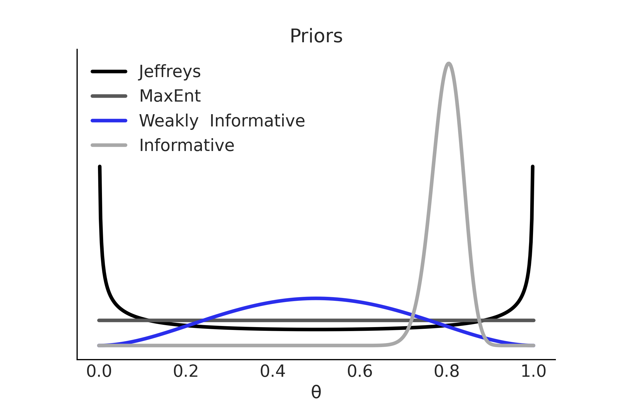
Fig. 1.11 Prior informativeness spectrum: While Jeffreys and MaxEnt priors are uniquely defined for a binomial likelihood, weakly informative and informative priors are not and instead depend on previous information and practitioner’s modeling decisions.

Because weakly-informative priors work to keep the posterior distribution within certain reasonable bounds, they are also known as regularizing priors. Regularization is a procedure of adding information with the aim of solving an ill-posed problem or to reduce the chance of overfitting and priors offer a principled way of performing regularization.

In this book, more often than not, we will use weakly-informative priors. Sometimes the prior will be used in a model without too much justification, simply because the focus of the example may be related to other aspects of the Bayesian modeling workflow. But we will also show some examples of using prior predictive checks to help us calibrate our priors.

Overfitting

Overfitting occurs when a model generates predictions very close to the limited dataset used to fit it, but it fails to fit additional data and/or predict future observations reasonably well. That is it fails to generalize its predictions to a wider set of possible observations. The counterpart of overfitting is underfitting, which is when a model fails to adequately capture the underlying structure of the data. We will discuss more about there topics in Sections Model Comparison and Information Criterion.

1.4.5. Using Prior Predictive Distributions to Assess Priors

When evaluating the choice of priors, the prior predictive distribution shown in Say Yes to Automating Inference, Say No to Automated Model Building is a handy tool. By sampling from the prior predictive distribution, the computer does the work of translating choices made in the parameter space into samples in the observed variable space. Thinking in terms of observed values is generally easier than thinking in terms of the model’s parameters which makes model evaluation easier. Following a Beta Binomial model, instead of judging whether a particular value of \(\theta\) is plausible, prior predictive distributions allow us to judge whether a particular number of successes is plausible. This becomes even more useful for complex models where parameters get transformed through many mathematical operations or multiple priors interact with each other. Lastly, computing the prior predictive could help us ensure our model has been properly written and is able to run in our probabilistic programming language and can even help us to debug our model. In the following chapters, we will see more concrete examples of how to reason about prior predictive samples and use them to choose reasonable priors.

1.5. Exercises

Problems are labeled Easy (E), Medium (M), and Hard (H).

1E1. As we discussed, models are artificial representations used to help define and understand an object or process. However, no model is able to perfectly replicate what it represents and thus is deficient in some way. In this book we focus on a particular type of models, statistical models. What are other types of models you can think of? How do they aid understanding of the thing that is being modeled? How are they deficient?

1E2. Match each of these verbal descriptions to their corresponding mathematical expression:

1. The probability of a parameter given the observed data

2. The distribution of parameters before seeing any data

3. The plausibility of the observed data given a parameter value

4. The probability of an unseen observation given the observed data

5. The probability of an unseen observation before seeing any data

1E3. From the following expressions, which one corresponds to the sentence, The probability of being sunny given that it is July 9th of 1816?

1. \(p(\text{sunny})\)

2. \(p(\text{sunny} \mid \text{July})\)

3. \(p(\text{sunny} \mid \text{July 9th of 1816})\)

4. \(p(\text{July 9th of 1816} \mid \text{sunny})\)

5. \(p(\text{sunny}, \text{July 9th of 1816}) / p(\text{July 9th of 1816})\)

1E4. Show that the probability of choosing a human at random and picking the Pope is not the same as the probability of the Pope being human. In the animated series Futurama, the (Space) Pope is a reptile. How does this change your previous calculations?

1E5. Sketch what the distribution of possible observed values could be for the following cases:

1. The number of people visiting your local cafe assuming Poisson distribution

2. The weight of adult dogs in kilograms assuming a Uniform distribution

3. The weight of adult elephants in kilograms assuming Normal distribution

4. The weight of adult humans in pounds assuming skew Normal distribution

1E6. For each example in the previous exercise, use SciPy to specify the distribution in Python. Pick parameters that you believe are reasonable, take a random sample of size 1000, and plot the resulting distribution. Does this distribution look reasonable given your domain knowledge? If not adjust the parameters and repeat the process until they seem reasonable.

1E7. Compare priors \(\text{Beta}(0.5, 0.5)\), \(\text{Beta}(1, 1)\), \(\text{Beta}(1, 4)\). How do the priors differ in terms of shape?

1E8. Rerun Code Block binomial_update but using two Beta-priors of your choice. Hint: you may what to try priors with \(\alpha \neq \beta\) like \(\text{Beta}(2, 5)\).

1E9. Try to come up with new constraints in order to obtain new Max-Ent distributions (Code Block max_ent_priors)

1E10. In Code Block metropolis_hastings, change the value of can_sd and run the Metropolis-Hastings sampler. Try values like 0.001 and 1.

1. Compute the mean, SD, and HDI and compare the values with those in the book (computed using can_sd=0.05). How different are the estimates?

2. Use the function az.plot_posterior.

1E11. You need to estimate the weights of blue whales, humans, and mice. You assume they are normally distributed, and you set the same prior \(\mathcal{HN}(200\text{kg})\) for the variance. What type of prior is this for adult blue whales? Strongly informative, weakly informative, or non-informative? What about for mice and for humans? How does informativeness of the prior correspond to our real world intuitions about these animals?

1E12. Use the following function to explore different combinations of priors (change the parameters a and b) and data (change heads and trials). Summarize your observations.

def posterior_grid(grid=10, a=1, b=1, heads=6, trials=9):
    grid = np.linspace(0, 1, grid)
    prior = stats.beta(a, b).pdf(grid)
    likelihood = stats.binom.pmf(heads, trials, grid)
    posterior = likelihood * prior
    posterior /= posterior.sum()
    _, ax = plt.subplots(1, 3, sharex=True, figsize=(16, 4))
    ax[0].set_title(f"heads = {heads}\ntrials = {trials}")
    for i, (e, e_n) in enumerate(zip(
            [prior, likelihood, posterior],
            ["prior", "likelihood", "posterior"])):
        ax[i].set_yticks([])
        ax[i].plot(grid, e, "o-", label=e_n)
        ax[i].legend(fontsize=14)


interact(posterior_grid,
    grid=ipyw.IntSlider(min=2, max=100, step=1, value=15),
    a=ipyw.FloatSlider(min=1, max=7, step=1, value=1),
    b=ipyw.FloatSlider(min=1, max=7, step=1, value=1),
    heads=ipyw.IntSlider(min=0, max=20, step=1, value=6),
    trials=ipyw.IntSlider(min=0, max=20, step=1, value=9))

1E13. Between the prior, prior predictive, posterior, and posterior predictive distributions which distribution would help answer each of these questions. Some items may have multiple answers.

1. How do we think is the distribution of parameters values before seeing any data?

2. What observed values do we think we could see before seeing any data?

3. After estimating parameters using a model what do we predict we will observe next?

4. What parameter values explain the observed data after conditioning on that data?

5. Which can be used to calculate numerical summaries, such as the mean, of the parameters?

6. Which can can be used to visualize a Highest Density Interval?

1M14. Equation (1.1) contains the marginal likelihood in the denominator, which is difficult to calculate. In Equation (1.3) we show that knowing the posterior up to a proportional constant is sufficient for inference. Show why the marginal likelihood is not needed for the Metropolis-Hasting method to work. Hint: this is a pen and paper exercise, try by expanding Equation (1.9).

1M15. In the following definition of a probabilistic model, identify the prior, the likelihood, and the posterior:

(1.22)\[\begin{split}\begin{split} Y \sim \mathcal{N}(\mu, \sigma)\\ \mu \sim \mathcal{N}(0, 1)\\ \sigma \sim \mathcal{HN}(1)\\ \end{split}\end{split}\]

1M16. In the previous model, how many parameters will the posterior have? Compare your answer with that from the model in the coin-flipping problem in Equation (1.10).

1M17. Suppose that we have two coins; when we toss the first coin, half of the time it lands tails and half of the time on heads. The other coin is a loaded coin that always lands on heads. If we choose one of the coins at random and observe a head, what is the probability that this coin is the loaded one?

1M18. Modify Code Block metropolis_hastings_sampler_rvs to generate random samples from a Poisson distribution with parameters of your choosing. Then modify Code Blocks metropolis_hastings_sampler and metropolis_hastings to generate MCMC samples estimating your chosen parameters. Test how the number of samples, MCMC iterations, and initial starting point affect convergence to your true chosen parameter.

1M19. Assume we are building a model to estimate the mean and standard deviation of adult human heights in centimeters. Build a model that will make this estimation. Start with Code Block beta_binom and change the likelihood and priors as needed. After doing so then

1. Sample from the prior predictive. Generate a visualization and numerical summary of the prior predictive distribution

2. Using the outputs from (a) to justify your choices of priors and likelihoods

1M20. From domain knowledge you have that a given parameter can not be negative, and has a mean that is roughly between 3 and 10 units, and a standard deviation of around 2. Determine two prior distributions that satisfy these constraints using Python. This may require trial and error by drawing samples and verifying these criteria have been met using both plots and numerical summaries.

1M21. A store is visited by \(n\) customers on a given day. The number of customers that make a purchase \(Y\) is distributed as \(\text{Bin}(n, \theta)\), where \(\theta\) is the probability that a customer makes a purchase. Assume we know \(\theta\) and the prior for \(n\) is \(\text{Pois}(4.5)\).

1. Use PyMC3 to compute the posterior distribution of \(n\) for all combinations of \(Y \in {0, 5, 10}\) and \(\theta \in {0.2, 0.5}\). Use az.plot_posterior to plot the results in a single plot.

2. Summarize the effect of \(Y\) and \(\theta\) on the posterior

1H22. Modify Code Block metropolis_hastings_sampler_rvs to generate samples from a Normal Distribution, noting your choice of parameters for the mean and standard deviation. Then modify Code Blocks metropolis_hastings_sampler and metropolis_hastings to sample from a Normal model and see if you can recover your chosen parameters.

1H23. Make a model that estimates the proportion of the number of sunny versus cloudy days in your area. Use the past 5 days of data from your personal observations. Think through the data collection process. How hard is it to remember the past 5 days. What if needed the past 30 days of data? Past year? Justify your choice of priors. Obtain a posterior distribution that estimates the proportion of sunny versus cloudy days. Generate predictions for the next 10 days of weather. Communicate your answer using both numerical summaries and visualizations.

1H24. You planted 12 seedlings and 3 germinate. Let us call \(\theta\) the probability that a seedling germinates. Assuming \(\text{Beta}(1, 1)\) prior distribution for \(\theta\).

1. Use pen and paper to compute the posterior mean and standard deviation. Verify your calculations using SciPy.

2. Use SciPy to compute the equal-tailed and highest density 94% posterior intervals.

3. Use SciPy to compute the posterior predictive probability that at least one seedling will germinate if you plant another 12 seedlings.

After obtaining your results with SciPy repeat this exercise using PyMC3 and ArviZ

---

[1]

If you want to be more general you can even say that everything is a probability distribution as a quantity you assume to know with arbitrary precision that can be described by a Dirac delta function.

[2]

Some authors call these quantities latent variables and reserve the name parameter to identify fixed, but unknown, quantities.

[3]

Alternatively you can think of this in terms of certainty or information, depending if you are a glass half empty or glass half full person.

[4]

Sometimes the word distribution will be implicit, this commonly occurs when discussing these topics.

[5]

Here we are using experiment in the broad sense of any procedure to collect or generate data.

[6]

https://xkcd.com/2117/

[7]

Technically we should talk about the expectation of a random variable. See Section Expectations for details.

[8]

See detailed balance at Sections Markov Chains and Metropolis-Hastings.

[9]

For a more extensive discussion about inference methods you should read Section [Inference Methods and references therein.

[10]

This is sometimes referred to as a kernel in other Universal Inference Engines.

[11]

You can use ArviZ plot_trace function to get a similar plot. This is how we will do in the rest of the book.

[12]

Notice that in principle the number of possible intervals containing a given proportion of the total density is infinite.

[13]

For more examples check https://en.wikipedia.org/wiki/Conjugate_prior#Table_of_conjugate_distributions

[14]

Except, the ones happening in your brain.

[15]

For example, a regularized linear regression with a L2 regularization is the same as using a Gaussian prior on the coefficient.

[16]

For example, if we have samples from the posterior, then we can plug those samples of \(\theta\) into \(\kappa = \frac{\theta}{1-\theta}\).

[17]

https://en.wikipedia.org/wiki/Likelihood_principle

[18]

See Section Entropy for more details.

[19]

Wikipedia has a longer list at https://en.wikipedia.org/wiki/Maximum_entropy_probability_distribution#Other_examples

[20]

Even when the definition of such priors will require more context than the one provided, we still think the example conveys a useful intuition, that will be refined as we progress through this book.