4. Extending Linear Models

A common trope in a sales pitch is the phrase “But wait! There is more!” In the lead up an audience is shown a product that incredibly seems to do it all, but somehow the salesperson shows off another use case for the already incredibly versatile tool. This is what we say to you about linear regression. In Chapter 3 we show a variety of ways to use and extend linear regression. But there is still a lot more we can do with linear models. From covariate transformation, varying variance, to multilevel models: each of these ideas provide extra flexibility to use linear regressions in an even wider set of circumstances.

4.1. Transforming Covariates

In Chapter 3 we saw that with a linear model and an identity link function, a unit change in \(x_i\) led to a \(\beta_i\) change in the expected response variable \(Y\), at any value of \(X_i\). Then we saw how Generalized Linear Models can be created by changing the likelihood function (e.g. from a Gaussian to Bernoulli), which in general requires a change in the link function.

Another useful modification, to the vanilla linear model, is to transform the covariates \(\mathbf{X}\), in order to make the relationship between \(\mathbf{X}\) and \(Y\) nonlinear. For example, we may assume that a square-root-unit change or log-unit change, etc. in \(x_i\) led to a \(\beta_i\) change in the expected response variable \(Y\). We can note express mathematically by extending Equation (3.2) with an additional term, \(f(.)\), which indicates an arbitrary transformation applied to each covariate \((X_i)\):

(4.1)\[\begin{split}\begin{split} \mu =& \beta_0 + \beta_1 f_1(X_1) + \dots + \beta_m f_m(X_m) \\ Y \sim& \mathcal{N}(\mu, \sigma) \end{split}\end{split}\]

In most of our previous examples \(f(.)\) was present but was the identity transformation. In a couple of the previous examples we centered the covariates to make the coefficient easier to interpret and the centering operation is one type of covariate transformation. However, \(f(.)\) can be any arbitrary transformation. To illustrate, let us borrow an example from Bayesian Analysis with Python [41] and create a model for the length of babies. First we will load the data and plot in Code Block babies_data and plot the age and month in Fig. 4.1.

Listing 4.1 babies_data

babies = pd.read_csv("../data/babies.csv")
# Add a constant term so we can use the dot product to express the intercept
babies["Intercept"] = 1

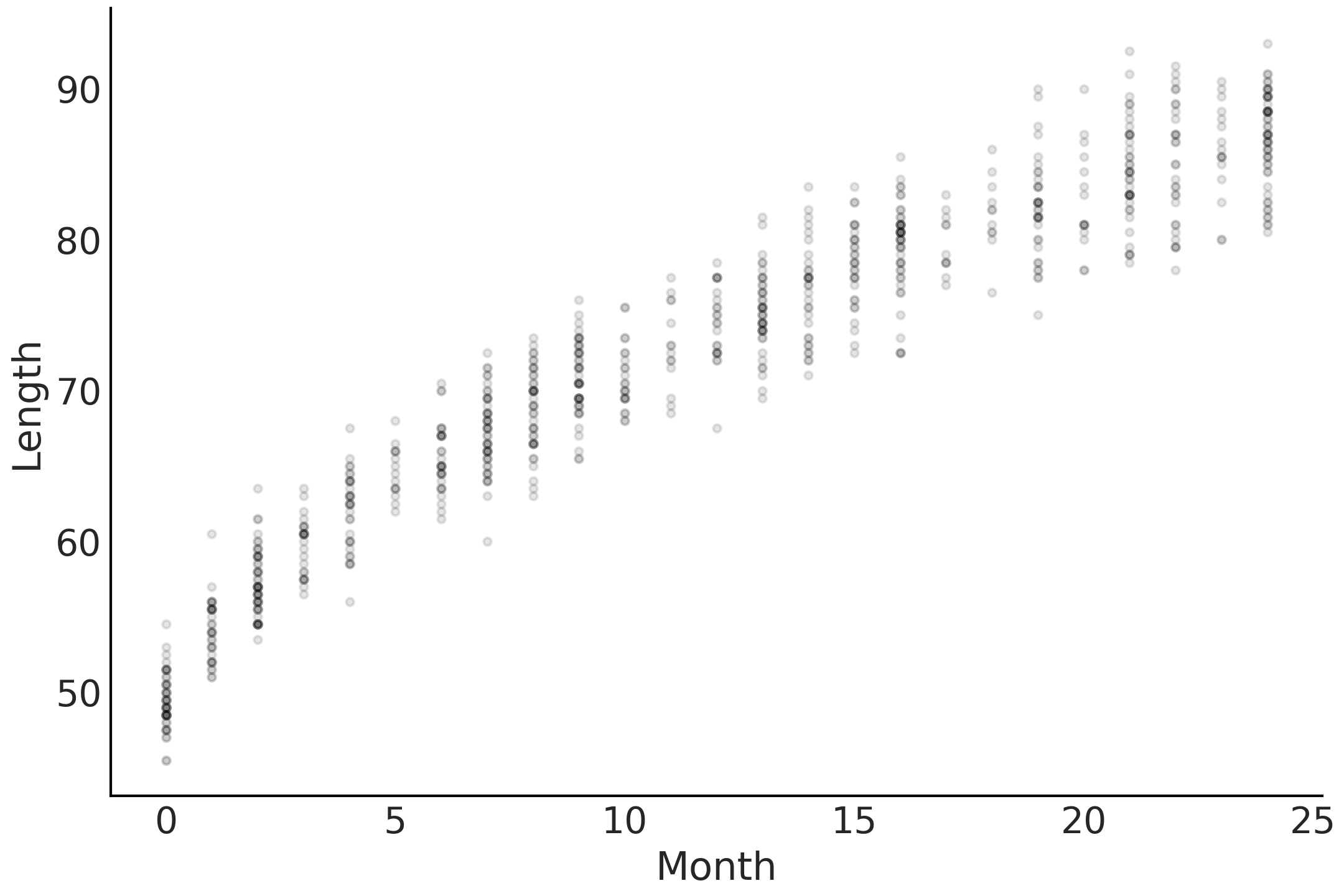
Fig. 4.1 Scatter plot of the nonlinear correlation between a baby’s age in months and observed, or measured, length.

Let us formulate a model in Code Block babies_linear which we can use to predict the length of the baby at each month of their childhood, as well as determine how quickly a child is growing per month. Note that this model formulation contains no transformations, and nothing we have not seen already in Chapter 3.

Listing 4.2 babies_linear

with pm.Model() as model_baby_linear:
    β = pm.Normal("β", sigma=10, shape=2)

    μ = pm.Deterministic("μ", pm.math.dot(babies[["Intercept", "Month"]], β))
    ϵ = pm.HalfNormal("ϵ", sigma=10)

    length = pm.Normal("length", mu=μ, sigma=ϵ, observed=babies["Length"])

    trace_linear = pm.sample(draws=2000, tune=4000)
    pcc_linear = pm.sample_posterior_predictive(trace_linear)
    inf_data_linear = az.from_pymc3(trace=trace_linear,
                                    posterior_predictive=pcc_linear)

model_linear faithfully gives us a linear growth rate as shown Fig. 4.2, estimating that babies will grow at the same rate of around 1.4 cm in each month of their observed childhood. However, it likely does not come as a surprise to you that humans do not grow at the same rate their entire lives and that they tend to grow more rapidly in the earlier stages of life. In other words the relationship between age and length is nonlinear. Looking more closely at Fig. 4.2 we can see some issues with the linear trend and the underlying data. The model tends to overestimate the length of babies close to 0 months of age, and over estimate length at 10 months of age, and then once again underestimate at 25 months of age. We asked for a straight line and we got a straight line even if the fit is not all that great.

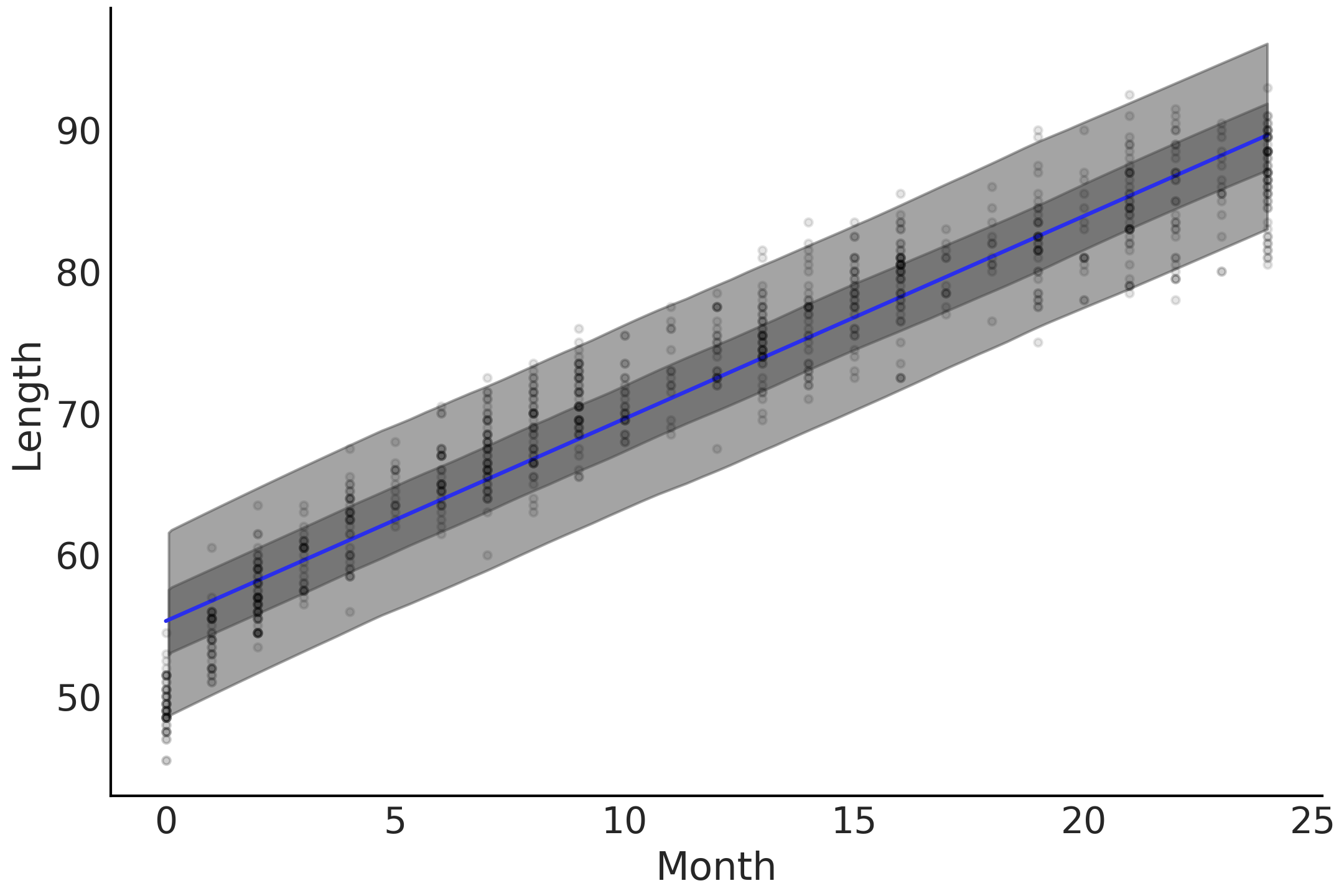
Fig. 4.2 A linear prediction of baby length, where the mean is the blue line, the dark gray is the 50% highest density interval of the posterior predictive and the light gray is the 94% highest density interval of the posterior predictive. The highest density interval around the mean line of fit covers most of the data points despite the predictions tend to be either biased high in the early months, 0 to 3, as well as late months, 22 to 25, and biased low in the middle at months 10 to 15.

Thinking back to our model choices, we still believe that at any age, or vertical slice of the observed data, the distribution of baby lengths being Gaussian-like, but the relationship between the month and mean length is nonlinear. Specifically, we decide that the nonlinearity generally follows the shape of a square root transformation on the month covariate which we write in model_sqrt in Code Block babies_transformed.

Listing 4.3 babies_transformed

with pm.Model() as model_baby_sqrt:
    β = pm.Normal("β", sigma=10, shape=2)

    μ = pm.Deterministic("μ", β[0] + β[1] * np.sqrt(babies["Month"]))
    σ = pm.HalfNormal("σ", sigma=10)

    length = pm.Normal("length", mu=μ, sigma=σ, observed=babies["Length"])
    inf_data_sqrt = pm.sample(draws=2000, tune=4000)

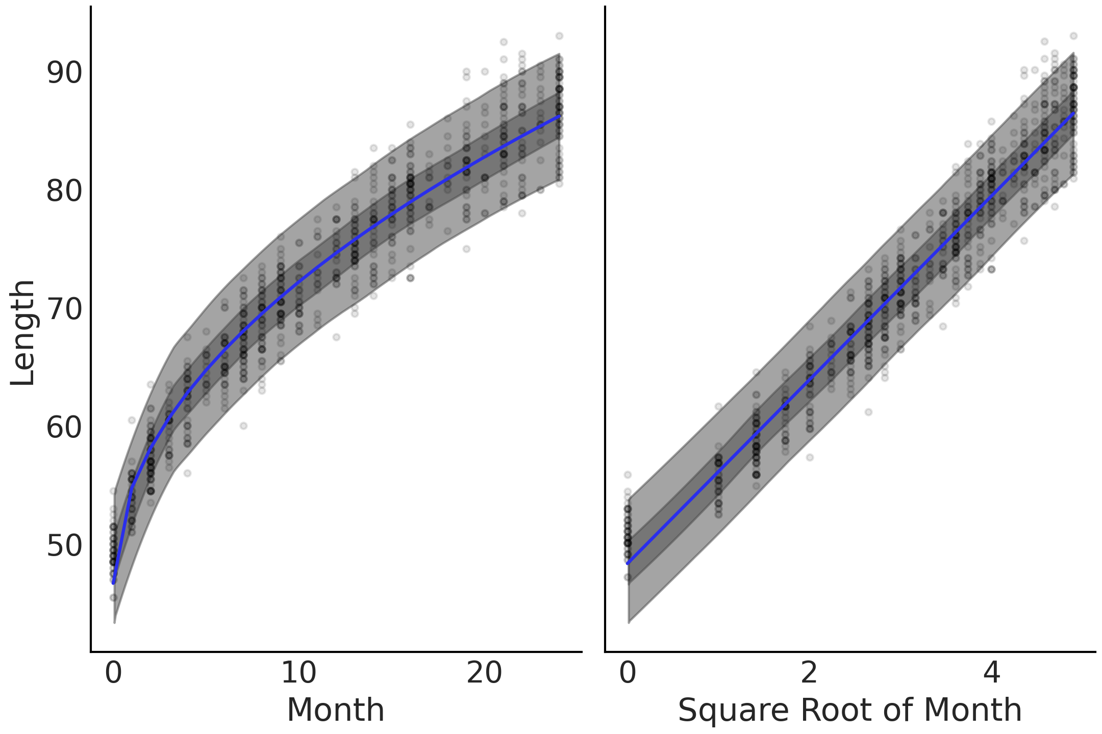
Fig. 4.3 Linear prediction with transformed covariate. On the left the x-axes is untransformed and on the right transformed. The linearization of the nonlinear growth rate is visible on the transformed axes on the right.

Plotting the fit of the means, along with bands representing the highest density interval of the expected length, yields Fig. 4.3, in which the means tends to fit the curve of the observed relationship. In addition to this visual check we can also use az.compare to verify the ELPD value for the nonlinear model. In your own analysis you can use any transformation function you would like. As with any model the important bit is to be able to justify your choice whatever it may be, and verify your results are reasonable using visual and numerical checks.

4.2. Varying Uncertainty

Thus far we have used linear models to model the mean of \(Y\) while assuming the variance of the residuals [1] is constant along the range of the response. However, this assumption of fixed variance is a modeling choice that may not be adequate. To account for changing uncertainty we can extend Equation (4.1) into:

(4.2)\[\begin{split}\begin{split} \mu =& \beta_0 + \beta_1 f_1(X_1) + \dots + \beta_m f_m(X_m) \\ \sigma =& \delta_0 + \delta_1 g_1(X_1) + \dots + \delta_m g_m(X_m) \\ Y \sim& \mathcal{N}(\mu, \sigma) \end{split}\end{split}\]

This second line estimating \(\sigma\) is very similar to our linear term which models the mean. We can use linear models to model parameters other than the mean/location parameter. For a concrete example let us expand model_sqrt defined in Code Block babies_transformed. We now assume that when children are young their lengths tend to cluster closely together, but as they age their lengths tend to become more dispersed.

Listing 4.4 babies_varying_variance

with pm.Model() as model_baby_vv:
    β = pm.Normal("β", sigma=10, shape=2)
    
    # Additional variance terms
    δ = pm.HalfNormal("δ", sigma=10, shape=2)

    μ = pm.Deterministic("μ", β[0] + β[1] * np.sqrt(babies["Month"]))
    σ = pm.Deterministic("σ", δ[0] + δ[1] * babies["Month"])

    length = pm.Normal("length", mu=μ, sigma=σ, observed=babies["Length"])
    
    trace_baby_vv = pm.sample(2000, target_accept=.95)
    ppc_baby_vv = pm.sample_posterior_predictive(trace_baby_vv,
                                                 var_names=["length", "σ"])
    inf_data_baby_vv = az.from_pymc3(trace=trace_baby_vv,
                                     posterior_predictive=ppc_baby_vv)

To model increasing dispersion of the length of as the observed children get older we changed our definition of \(\sigma\) from a fixed value to a value that varies as a function of age. In other words we change the model assumption from homoscedastic, that is having constant variance, to heteroscedastic, that is having varying variance. In our model, defined in Code Block babies_varying_variance all we need to do is change the expression defining \(\sigma\) of our model and the PPL handle the estimation for us . The results of this model are plotted in Fig. 4.4.

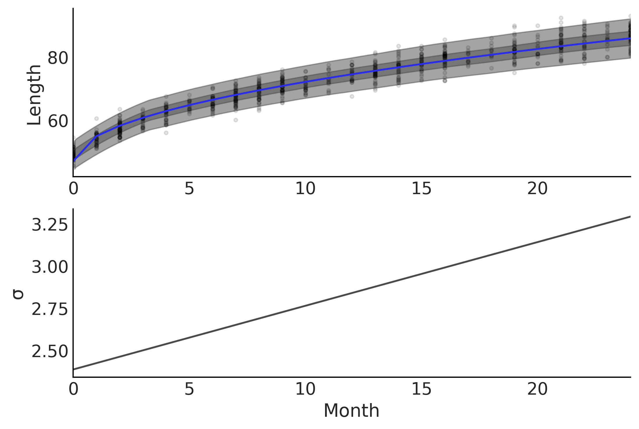
Fig. 4.4 Two plots showing parameter fits of baby month versus length. In the top plot the expected mean prediction, represented with a blue line, is identical to Fig. 4.3, however, the HDI intervals of the posterior are non-constant. The bottom graph plots the expected error estimate \(\sigma\) as a function of age in months. Note how the expected estimate of error increases as months increase.

4.3. Interaction Effects

In all our models thus far, we have assumed the effect of one covariate to the response variable is independent of any other covariates. This is not always the case. Consider a situation where we want to model ice cream sales for a particular town. We might say if there are many ice cream shops, more ice cream is available so we expect a large volume of ice cream purchases. But if this town in a cold climate with an average daily temperature of -5 degrees Celsius, we doubt there would be many sales of ice cream. However, in the converse scenario if the town was in a hot desert with average temperature of 30 degrees Celsius, but there are no ice cream stores, sales of ice cream would also be low. It is only when there is both hot weather and there are many places to buy ice cream that we expect an increased volume of sales. Modeling this kind of joint phenomena requires that we introduce an interaction effect, where the effect of one covariate on the output variable depends on the value of other covariates. Thus, if we assume covariates to contribute independently (as in a standard linear regression model), we will not be able to fully explain the phenomena. We can express an interaction effect as:

(4.3)\[\begin{split}\begin{split} \mu =& \beta_0 + \beta_1 X_1 + \beta_2 X_2 + \beta_3 X_1X_2\\ Y \sim& \mathcal{N}(\mu, \sigma) \end{split}\end{split}\]

where \(\beta_3\) is the coefficient for the interaction term \(X_1X_2\). There are other ways to introduce interactions but computing the products of original covariates is a very widely used option. Now that we have defined what an interaction effect is we can by contrast define a main effect, as the effect of one covariate on the dependent variable while ignoring all other covariates.

To illustrate let us use another example where we model the amount of tip a diner leaves as a function of the total bill in Code Block tips_no_interaction. This sounds reasonable as the amount of the tip is generally calculated as a percentage of the total bill with the exact percentage varying by different factors like the kind of place you are eating, the quality of the service, the country you are living, etc. In this example we are going to focus on the difference in tip amount from smokers versus non-smokers. In particular, we will study if there is an interaction effect between smoking and the total bill amount [2]. Just like Model penguin_mass_multi we can include smokers as an independent categorical variable in our regression.

Listing 4.5 tips_no_interaction

tips_df = pd.read_csv("../data/tips.csv")
tips = tips_df["tip"]
total_bill_c = (tips_df["total_bill"] - tips_df["total_bill"].mean())  
smoker = pd.Categorical(tips_df["smoker"]).codes

with pm.Model() as model_no_interaction:
    β = pm.Normal("β", mu=0, sigma=1, shape=3)
    σ = pm.HalfNormal("σ", 1)

    μ = (β[0] +
         β[1] * total_bill_c + 
         β[2] * smoker)

    obs = pm.Normal("obs", μ, σ, observed=tips)
    trace_no_interaction = pm.sample(1000, tune=1000)

Let us also create a model where we include an interaction term in Code Block tips_interaction.

Listing 4.6 tips_interaction

with pm.Model() as model_interaction:
    β = pm.Normal("β", mu=0, sigma=1, shape=4)
    σ = pm.HalfNormal("σ", 1)

    μ = (β[0]
       + β[1] * total_bill_c
       + β[2] * smoker
       + β[3] * smoker * total_bill_c
        )

    obs = pm.Normal("obs", μ, σ, observed=tips)
    trace_interaction = pm.sample(1000, tune=1000)

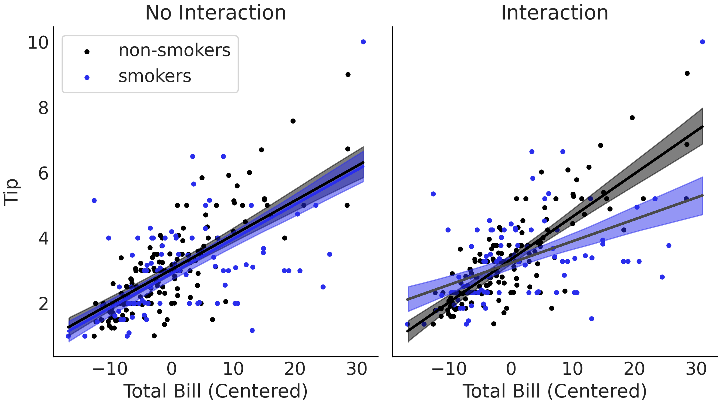
Fig. 4.5 Plots of linear estimates from our two tips models. On the right we show the non-interaction estimate from Code Block tips_no_interaction, where the estimated lines are parallel. On the left we show our model from Code Block tips_no_interaction that includes an interaction term between smoker or non-smoker and bill amount. In the interaction model the slopes between the groups are allowed to vary due to the added interaction term.

The difference is visible in Fig. 4.5. Comparing the non-interaction model on the left and the interaction on the right, the mean fitted lines are no longer parallel, the slopes for smokers and non-smokers are different! By introducing an interaction we are building a model that is effectively splitting the data, in this example into two categories, smokers and non-smokers. You may be thinking that it is a better idea to split the data manually and fit two separate models, one for the smokers and one for the non-smokers. Well, not so fast. One of the benefits of using interactions is that we are using all the available data to fit a single model, increasing the accuracy of the estimated parameters. For example, notice that by using a single model we are assuming that \(\sigma\) is not affected by the variable smoker and thus \(\sigma\) is estimated from both smokers and non-smokers, helping us to get a better estimation of this parameter. Another benefit is that we get an estimate of the size effect of the interaction. If we just split the data we are implicitly assuming the interaction is exactly 0, by modeling the interaction we get an estimate about how strong the interaction is. Finally, building a model with and without interactions for the same data to make easier to compare models using LOO. If we split the data we end-up with different models evaluated on different data, instead of different models evaluated on the same data, which is a requisite for using LOO. So in summary, while the primary difference in interaction effect models is flexibility in modeling different slopes per group, there are many additional benefits that arise from modeling all the data together.

4.4. Robust Regression

Outliers, as the name suggests, are observations that lie outside of the range “reasonable expectation”. Outliers are undesirable, as one, or few, of these data points could change the parameter estimation of a model significantly. There are a variety of suggested formal methods [42] of handling outliers, but in practice how outliers are handled is a choice a statistician has to make (as even the choice of a formal method is subjective). In general though there are at least two ways to address outliers. One is removing data using some predefined criteria, like 3 standard deviations or 1.5 times the interquartile range. Another strategy is choosing a model that can handle outliers and still provide useful results. In regression the latter are typically referred to as robust regression models, specifically to note these models are less sensitive to observations away from the bulk of the data. Technically speaking, robust regression are methods designed to be less affected by violations of assumptions by the underlying data-generating process. In Bayesian regression one example is changing the likelihood from a Gaussian distribution to a Student’s t-distribution.

Recall that Gaussian distributions are defined by two parameters typically known as location \(\mu\) and scale \(\sigma\). These parameters control the mean and standard deviation of the Gaussian distribution. Student’s t-distributions also have one parameter for the location and scale respectively [3]. However, there is an additional parameter, typically known as degrees of freedom \(\nu\). This parameter controls the weight of the tails of the Student’s t-distribution, as shown in Fig. 4.6. Comparing the 3 Student’s t-distributions against each other and the Normal distribution, the key difference is the proportion of the density in the tails versus the proportion at the bulk of the distributions. When \(\nu\) is small there is more mass distributed in the tails, as the value of \(\nu\) increases the proportion of density concentrated towards the bulk also increases and the Student’s t-distribution becomes closer and closer to the Gaussian. Practically speaking what this means is that values farther from the mean are more likely to occur when \(\nu\) is small. Which provides robustness to outliers when substituting a Gaussian likelihood with a Student’s t-distribution.

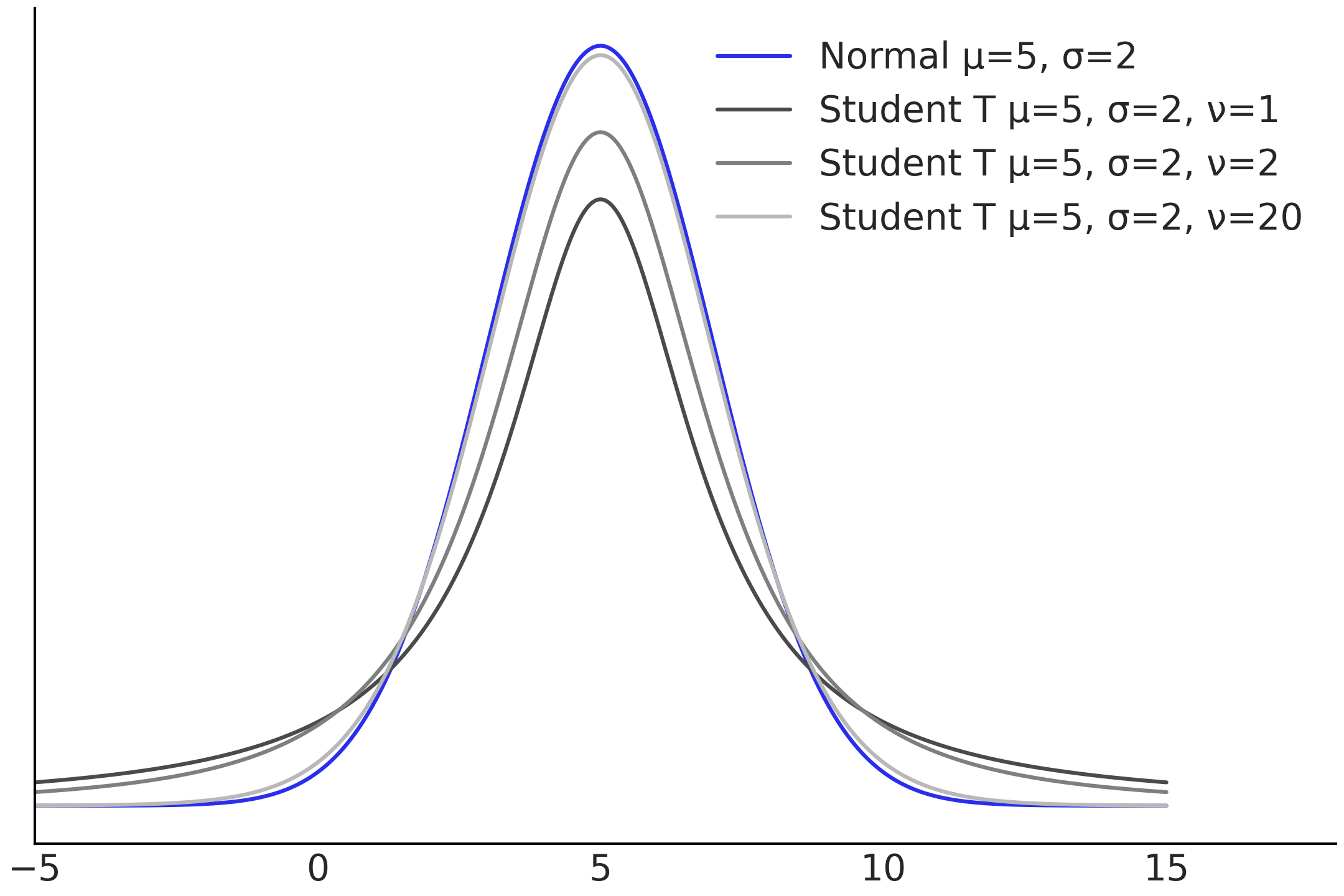
Fig. 4.6 Normal distribution, in blue, compared to 3 Student’s t-distributions with varying \(\nu\) parameters. The location and scale parameters are all identical, which isolates the effect \(\nu\) has on the tails of the distribution. Smaller values of \(\nu\) put more density into the tails of the distribution.

This can be shown in an example. Say you own a restaurant in Argentina and you sell empanadas [4]. Over time you have collected data on the number of customers per day and the total amount of Argentine pesos your restaurant has earned, as shown in Fig. 4.7. Most of the data points fall along a line, except during a couple of days where the number of empanadas sold per customer is much higher than the surrounding data points. These may be days of big celebration such as the 25th of May or 9th of July [5], where people are consuming more empanadas than usual.

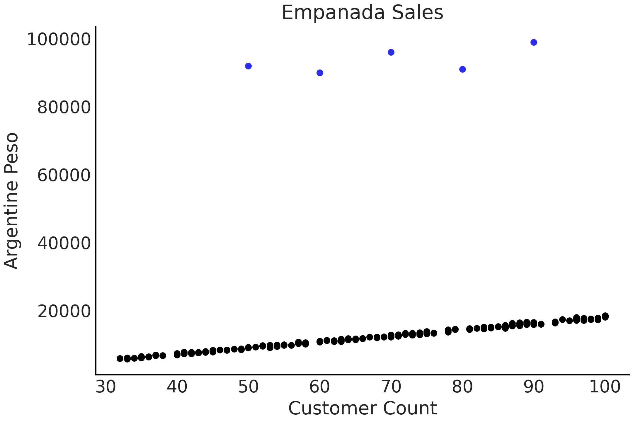
Fig. 4.7 Simulated data of number of customers plotted against the pesos returned. The 5 dots at the top of the chart are considered outliers.

Regardless of the outliers, we want to estimate the relationship between our customers and revenue. When plotting the data a linear regression seems appropriate, such as the one written in Code Block non_robust_regression which uses a Gaussian likelihood. After estimating the parameters we plot the mean regression in Fig. 4.8 at two different scales. In the lower plot note how the fitted regression line lies above all visible data points. In Table 4.1 we also can see the individual parameter estimates, noting in particular \(\sigma\) which at a mean value of 574 seems high when compared to the plot of the nominal data. With a Normal likelihood the posterior distribution has to “stretch” itself over the nominal observations and the 5 outliers, which affects the estimates. Additionally, note how the estimate of \(\sigma\) is quite wide compared to the plotted data in Fig. 4.8.

Listing 4.7 non_robust_regression

with pm.Model() as model_non_robust:
    σ = pm.HalfNormal("σ", 50)
    β = pm.Normal("β", mu=150, sigma=20)

    μ = pm.Deterministic("μ", β * empanadas["customers"])

    sales = pm.Normal("sales", mu=μ, sigma=σ, observed=empanadas["sales"])
    
    inf_data_non_robust = pm.sample()

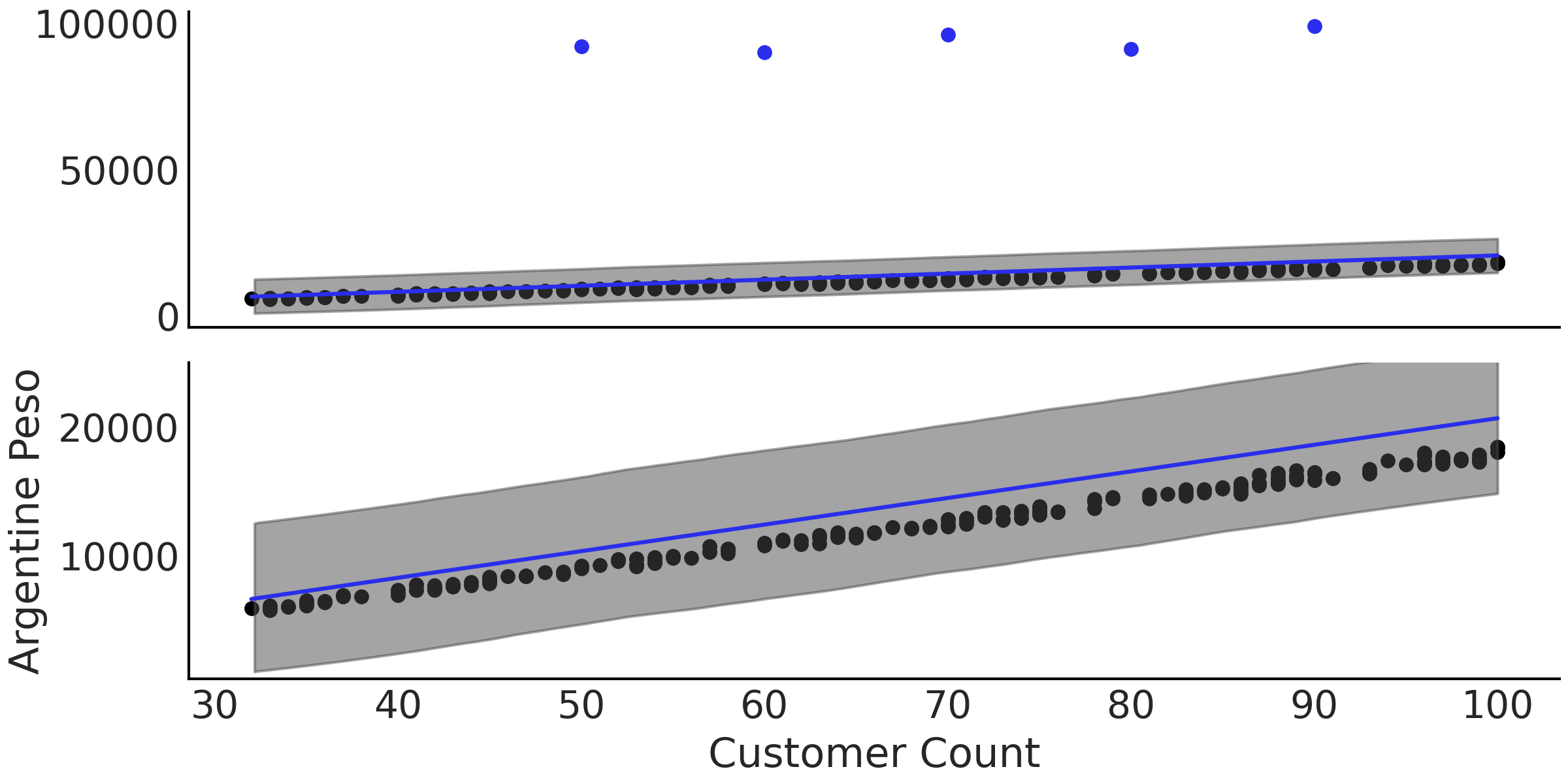
Fig. 4.8 A plot of the data, fitted regression line, and 94% HDI of model_non_robust from Code Block non_robust_regression at two scales, the top including the outliers, and the bottom focused on the regression itself. The systemic bias is more evident in bottom plot as the mean regression line is estimated to be above the nominal data points.

Table 4.1 Estimate of parameters for model non_robust_regression.

	mean	sd	hdi_3%	hdi_97%
\(\beta\)	207.1	2.9	201.7	212.5
\(\sigma\)	2951.1	25.0	2904.5	2997.7

We can run the same regression again but this time using the Student’s t-distribution as likelihood, shown in Code Block code_robust_regression. Note that the dataset has not changed and the outliers are still included. When inspecting the fitted regression line in Fig. 4.9 we can see that the fit falls between the nominal observed data points, closer to where we would expect. Inspecting the mean parameter estimates in Table 4.2 note the addition of the extra parameter \(\nu\). Furthermore we can see that the estimate of \(\sigma\) has fallen substantially from \(\approx\) 2951 pesos in the non-robust regression to \(\approx\) 152 pesos in the robust regression, note how this new estiamte is logically reasonable compared to the plotted data. The change in likelihood distribution shows that there is enough flexibility in the Student’s t-distribution to reasonably model the nominal data, despite the presence of outliers.

Listing 4.8 code_robust_regression

with pm.Model() as model_robust:
    σ = pm.HalfNormal("σ", 50)
    β = pm.Normal("β", mu=150, sigma=20)
    ν = pm.HalfNormal("ν", 20)

    μ = pm.Deterministic("μ", β * empanadas["customers"])
    
    sales = pm.StudentT("sales", mu=μ, sigma=σ, nu=ν,
                        observed=empanadas["sales"])

    inf_data_robust = pm.sample()

Table 4.2 Estimate of parameters for model robust_regression.

	mean	sd	hdi_3%	hdi_97%
\(\beta\)	179.6	0.3	179.1	180.1
\(\sigma\)	152.3	13.9	127.1	179.5
\(\nu\)	1.3	0.2	1.0	1.6

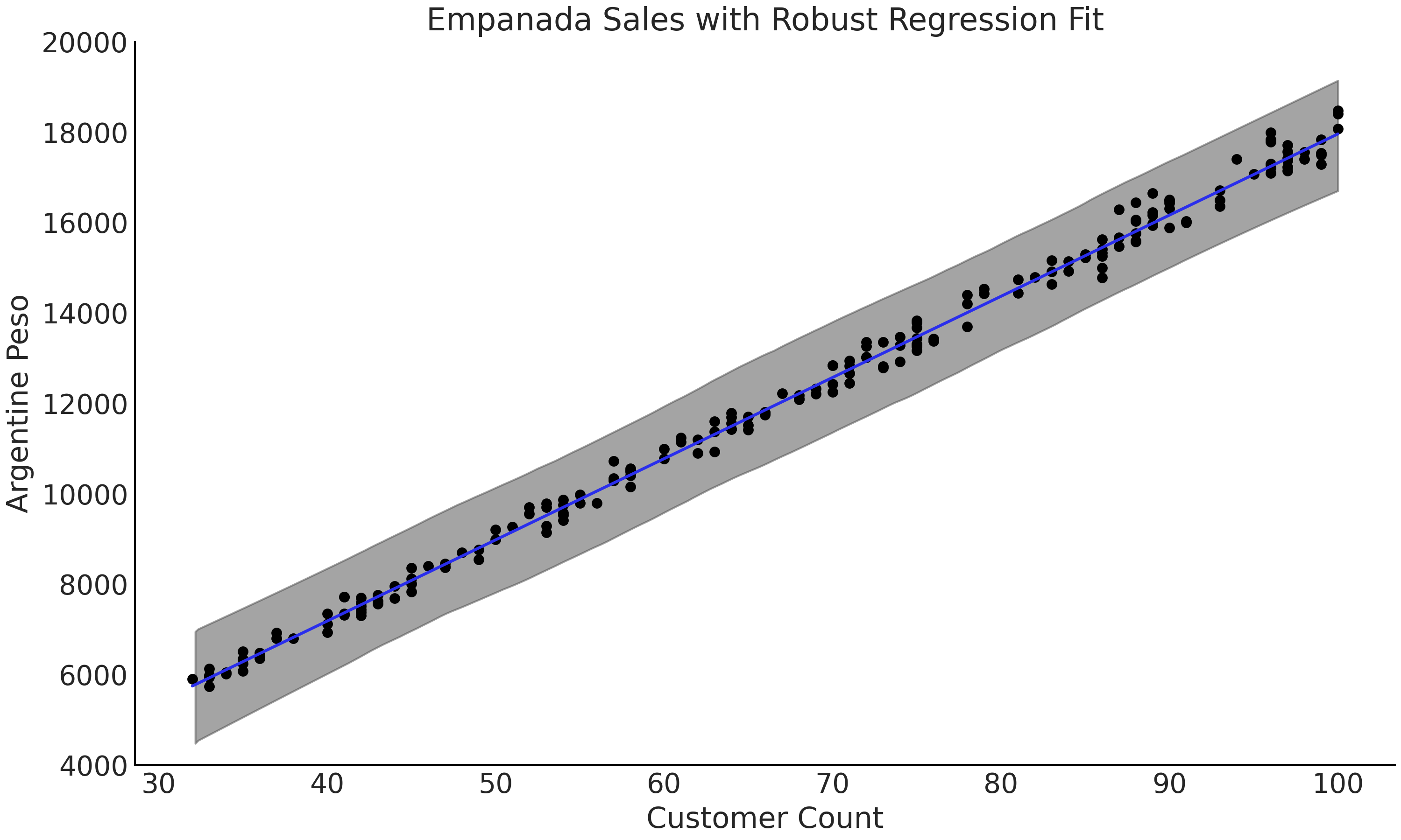
Fig. 4.9 A plot of the data, fitted regression line of model_robust and 94% HDI from Code Block code_robust_regression. The outliers are not plotted but are present in the data. The fitted line falls within the range of the nominal data points, particularly if compared to Fig. 4.8.

In this example the “outliers” are actually part of the problem we want to model, in the sense that they are not measurement error, data entry errors etc, but observations that can actually happened under certain conditions. Hence, it is ok to treat them as outliers if we want to model the average number of empanadas on a “regular” day, but it will lead to a disaster if we use this average to make plans for the next 25th of May or 9th of July. Therefore in this example the robust linear regression model is a trick to avoid explicitly modeling the high sales day which, if needed, will be probably better modeled using mixture model or a multilevel model.

Model adaptions for data considerations

Changing the likelihood to accommodate for robustness is just one example of a modification we can make to the model to better suit the observed data. For example, in detecting radioactive particle emission a zero count can arise because of a faulty sensor[43] (or some other measuring problem), or because there was actually no event to register. This unknown source of variation has the effect of inflating the count of zeros. A useful aid for this kind of problem is the class of models aptly named zero-inflated models which estimate the combined data generating process. For example, a Poisson likelihood, which will generally be a starting point for modeling counts, can be expanded into a zero-inflated Poisson likelihood. With such a likelihood we can better separate the counts generated from a Poisson process from those generated from the excess zero generating process.

Zero-inflated models are an example of handling a mixture of data, in which observations come from two or more groups, without knowledge of which observation belongs to which group. Actually, we can express another type of robust regression using a mixture likelihood, which assigns a latent label (outlier or not) to each data point.

In all of these situations and many more the bespoke nature of Bayesian models allows the modeler the flexibility to create a model that fits the situation, rather than having to fit a situation to a predefined model.

4.5. Pooling, Multilevel Models, and Mixed Effects

Often we have dataset that contain additional nested structures among the predictors, which gives some hierarchical way to group the data. We can also think of it as different data generation processes. We are going to use an example to illustrate this. Let us say you work at a restaurant company which sells salads. This company has a long-established business in some geographic markets and, due to customer demand, has just opened a location in a new market as well. You need to predict how many US dollars the restaurant location in this new market will earn each day for financial planning purposes. You have two datasets, 3 days of data for the sales of salads, as well as roughly a year’s worth of data on pizza and sandwich sales in the same market. The (simulated) data is shown in Fig. 4.10.

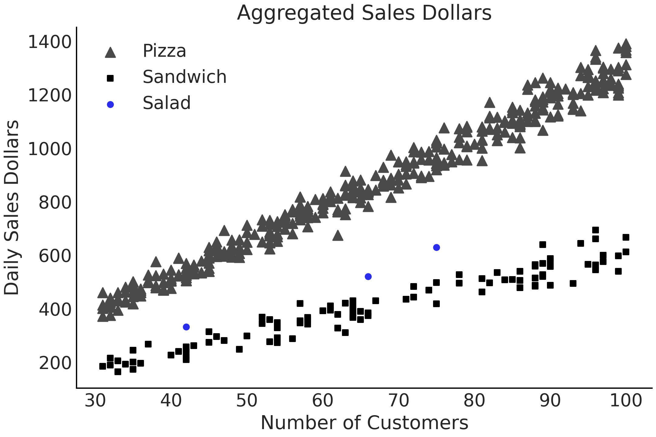
Fig. 4.10 A simulated dataset for a real world scenario. In this case an organization has 3 data points for the daily sales of salads, but has lots of data on the sales of pizza and sandwiches.

From both expert knowledge and data, there is agreement that there are similarities between the sales of these 3 food categories. They all appeal to the same type of customer, represent the same “food category” of quick to go food but they are not exactly the same either. In the following sections we will discuss how to model this similarity-yet-disimilarity but let us start with the simpler case, all groups are unrelated to each other.

4.5.1. Unpooled Parameters

We can create a regression model where we treat each group, in this case food category, as completely separated from the others. This is identical to running a separate regression for each category, and that is why we call it unpooled regression. The only difference to run separated regression is that we are writing a single model and estimating all coefficients at the same time. The relationship between parameters and groups is visually represented in Fig. 4.11 and in mathematical notation in Equation (4.4), where \(j\) is an index identifying each separated group.

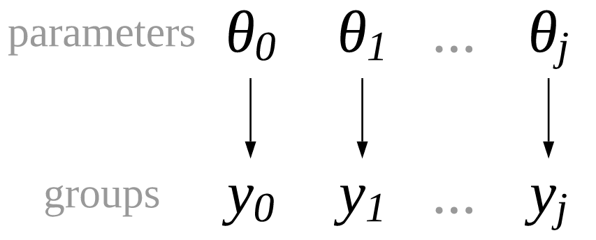
Fig. 4.11 An unpooled model where each group of observations, \(y_1, y_2, ..., y_j\) has its own set of parameters, independent from any other group.

(4.4)\[\begin{split}\begin{split} \beta_{mj} \sim& \overbrace{\mathcal{N}(\mu_{\beta m}, \sigma_{\beta m})}^{\text{Group-specific}}\\ \sigma_{j} \sim& \overbrace{\mathcal{HN}(\sigma_{\sigma})}^{\text{Group-specific}}\\ \mu_{j} =& \beta_{1j} X_1 + \dots + \beta_{mj} X_m \\ Y \sim& \mathcal{N}(\mu_{j}, \sigma_{j}) \end{split}\end{split}\]

The parameters are labeled as group-specific parameters to denote there is one dedicated to each group. The unpooled PyMC3 model, and some data cleaning, is shown in Code Block model_sales_unpooled and the block representation is shown in Fig. 4.12. We do not include an intercept parameter for the simple reason that if a restaurant has zero customers, total sales will also be zero, so there is neither any interest nor any need for the extra parameter.

Listing 4.9 model_sales_unpooled

customers = sales_df.loc[:, "customers"].values
sales_observed = sales_df.loc[:, "sales"].values
food_category = pd.Categorical(sales_df["Food_Category"])

with pm.Model() as model_sales_unpooled:
    σ = pm.HalfNormal("σ", 20, shape=3)
    β = pm.Normal("β", mu=10, sigma=10, shape=3)
    
    μ = pm.Deterministic("μ", β[food_category.codes] *customers)
    
    sales = pm.Normal("sales", mu=μ, sigma=σ[food_category.codes],
                      observed=sales_observed)
    
    trace_sales_unpooled = pm.sample(target_accept=.9)
    inf_data_sales_unpooled = az.from_pymc3(
        trace=trace_sales_unpooled, 
        coords={"β_dim_0":food_category.categories,
                "σ_dim_0":food_category.categories})

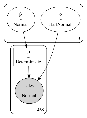
Fig. 4.12 A diagram of model_sales_unpooled. Note how the box around parameters \(\beta\) and \(\sigma\) has a three in the lower right, indicating that the model estimated 3 parameters each for \(\beta\) and \(\sigma\).

After sampling from model_sales_unpooled we can create forest plots of the parameter estimates as shown in Figures Fig. 4.13 and Fig. 4.14. Note how the estimate of \(\sigma\) for the salad food category is quite wide compared to the sandwich and pizza groups. This is what we would expect from our unpooled model when we have large amounts of data for some of the categories, but much less for others.

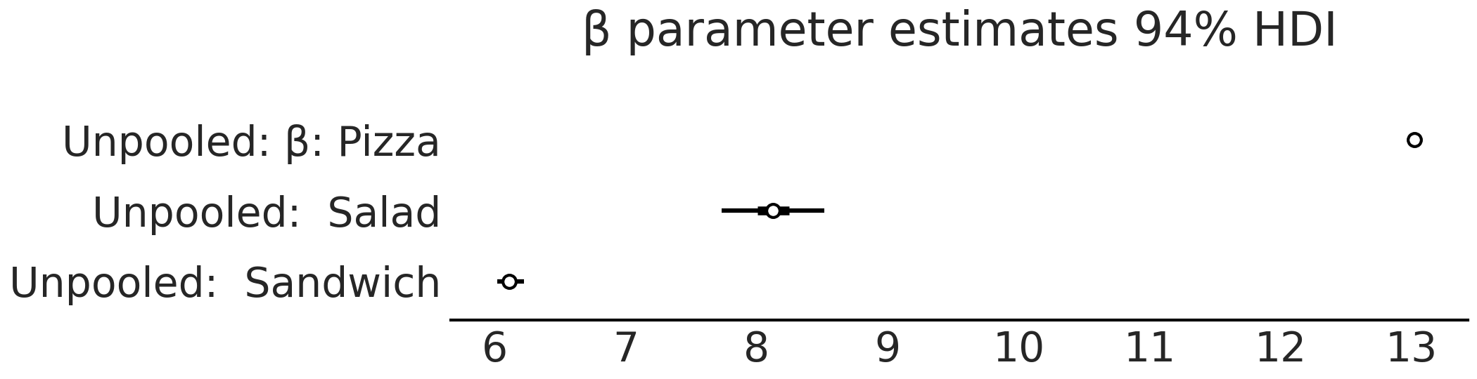
Fig. 4.13 Forest plot of the \(\beta\) parameter estimates model_sales_unpooled. As expected the estimate of the \(\beta\) coefficient for the salads group is the widest as this group has the least amount of data.

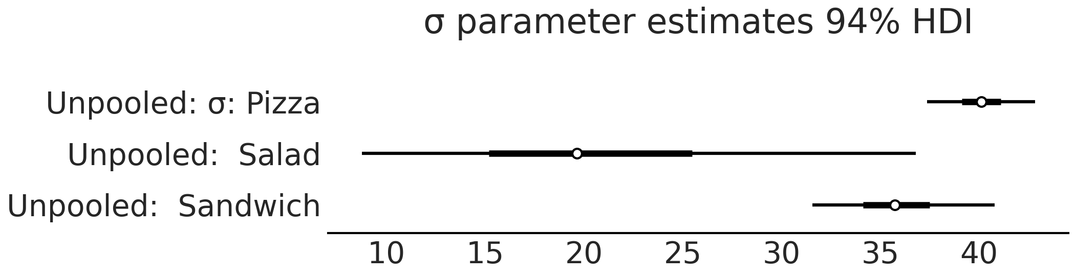
Fig. 4.14 Forest plot of the \(\sigma\) parameter estimates model_sales_unpooled. Like Fig. 4.13 the estimate of the variation of sales, \(\sigma\), is largest for the salads group as there are not as many data points relative to the pizza and sandwich groups.

The unpooled model is no different than if we have created three separated models with subsets of the data, exactly as we did in Section Comparing Two (or More) Groups, where the parameters of each group were estimated separately so we can consider the unpooled model architecture syntactic sugar for modeling independent linear regressions of each group. More importantly now we can use the unpooled model and the estimated parameters from it as a baseline to compare other models in the following sections, particularly to understand if the extra complexity is justified.

4.5.2. Pooled Parameters

If there are unpooled parameters, you might guess there are pooled parameters and you would be correct. As the name suggests pooled parameters are ones where the group distinction is ignored. Conceptually, this type of model is shown in Fig. 4.15 were each group shares the same parameters and thus we also refer to them as common parameters.

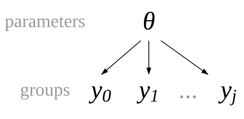
Fig. 4.15 A pooled model where each group of observations, \(y_1, y_2, ..., y_j\) shares parameters.

For our restaurant example, the model is written in Equation (4.5) and Code Block model_sales_pooled. The GraphViz representation is also shown in Fig. 4.12.

(4.5)\[\begin{split}\begin{split} \beta \sim& \overbrace{\mathcal{N}(\mu_{\beta}, \sigma_{\beta})}^{\text{Common}}\\ \sigma \sim& \overbrace{\mathcal{HN}(\sigma_{\sigma})}^{\text{Common}}\\ \mu =& \beta_{1} X_{1} + \dots + \beta_{m} X_{m} \\ Y \sim& \mathcal{N}(\mu, \sigma) \end{split}\end{split}\]

Listing 4.10 model_sales_pooled

with pm.Model() as model_sales_pooled:
    σ = pm.HalfNormal("σ", 20)
    β = pm.Normal("β", mu=10, sigma=10)

    μ = pm.Deterministic("μ", β * customers)
    
    sales = pm.Normal("sales", mu=μ, sigma=σ,
                      observed=sales_observed)
                        
    inf_data_sales_pooled = pm.sample()

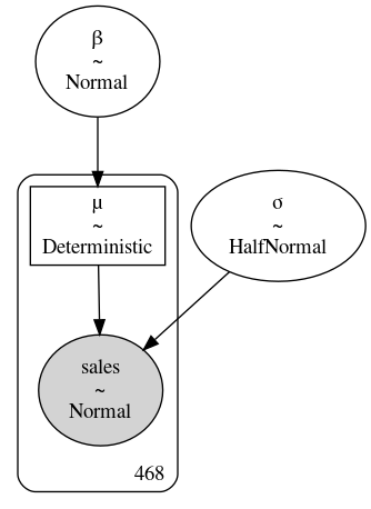
Fig. 4.16 Diagram of model_sales_pooled. Unlike Fig. 4.12 there is only one instance of \(\beta\) and \(\sigma\).

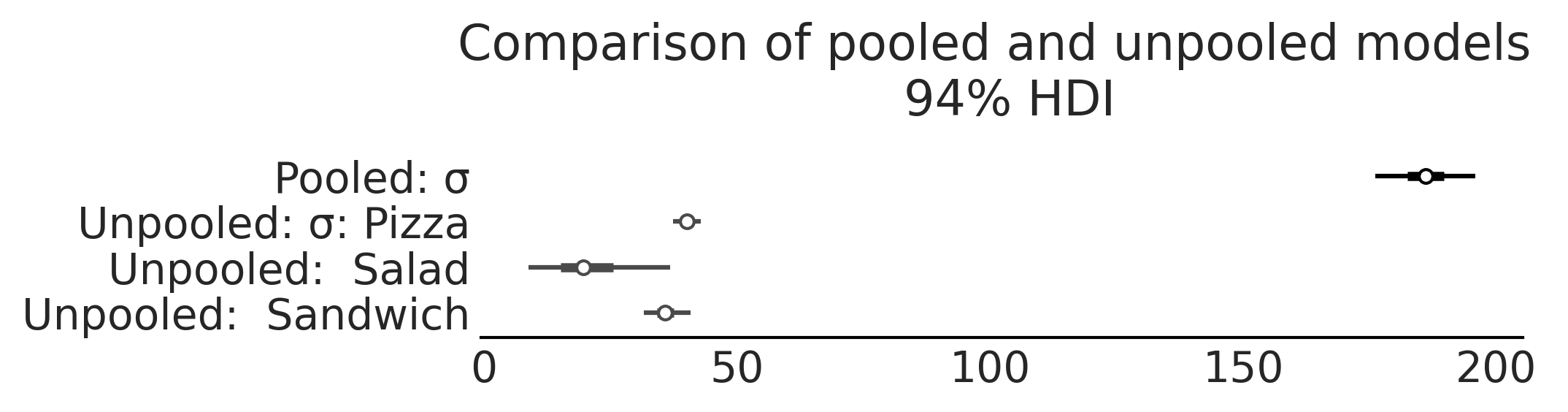
Fig. 4.17 A comparison of the estimates of the \(\sigma\) parameter from model_pooled_sales and model_unpooled_sales. Note how we only get one estimate of \(\sigma\) that is much higher compared to the unpooled model as the single linear fit estimated must capture the variance in the pooled data.

The benefit of the pooled approach is that more data will be used to estimate each parameter. However, this means we cannot understand each group individually, just all food categories as a whole. Looking at Fig. 4.18, our estimates \(\beta\) and \(\sigma\) are not indicative of any particular food group as the model is grouping together data with very different scales. Compare the value of \(\sigma\) with the ones from the unpooled model in Fig. 4.17. When plotting the regression in Fig. 4.18 we can see that a single line, despite being informed by more data than any single group, fails to fit any one group well. This result implies that the differences in the groups are too large to ignore and thus pooling the data it is not particularly useful for our intended purpose.

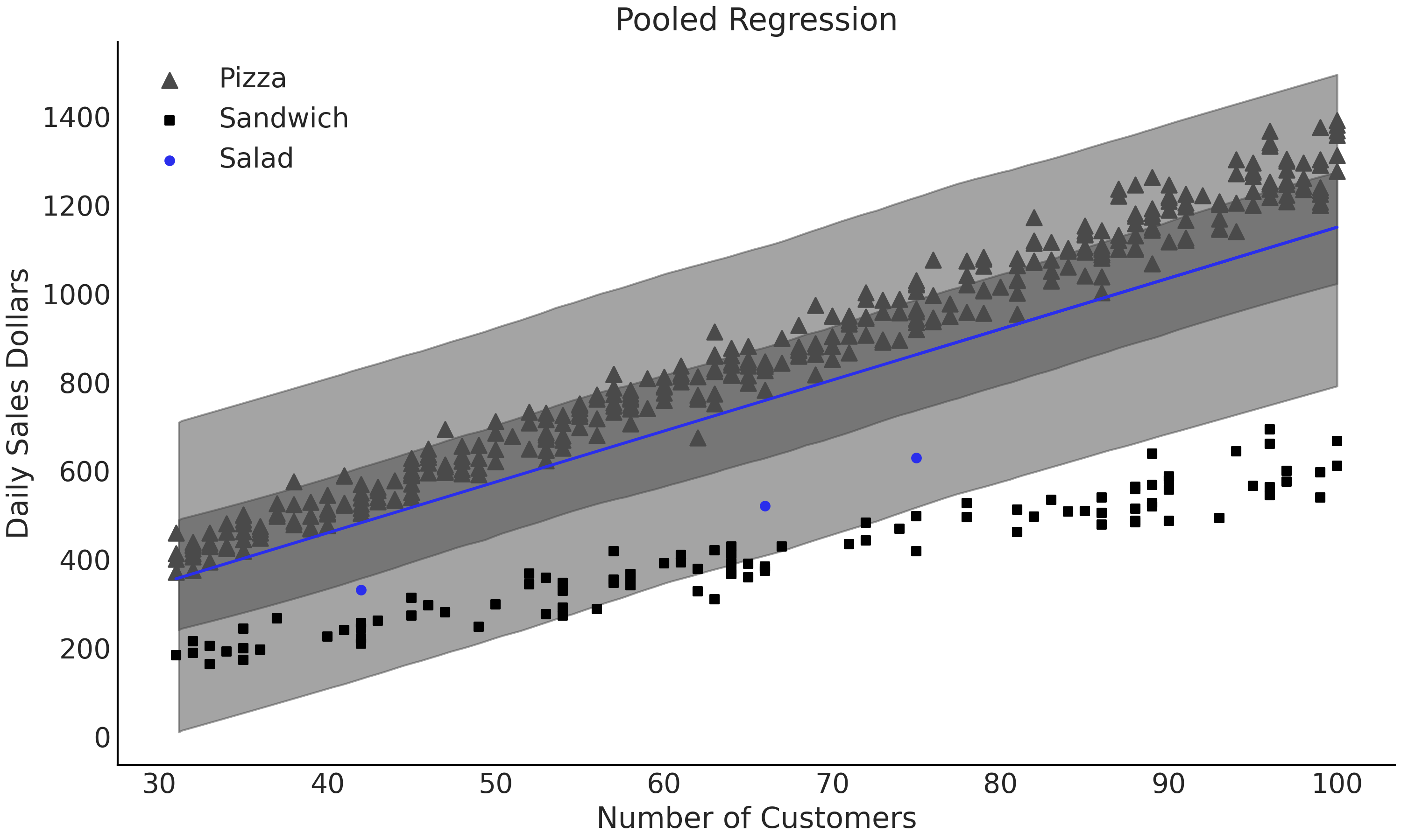
Fig. 4.18 Linear regression model_sales_pooled where all the data is pooled together. Each of the parameters is estimated using all the data but we end up with poor estimates of each individual group’s behavior as a 2 parameter model cannot generalize well enough to capture the nuances of each group.

4.5.3. Mixing Group and Common Parameters

In the unpooled approach we get the benefit of preserving the differences in our groups, and thus getting an estimated set of parameters for each group. In the pooled approach we get the benefit of utilizing all the data to estimate a single set of parameters, and thus more informed, albeit more generic, estimates. Fortunately we are not forced to pick just one option or the other. We can mix these two concepts in a single model shown in Equation (4.6). In this formulation we have decided to keep the estimate of \(\beta\) group specific, or unpooled, and to use a common, or pooled, \(\sigma\). In our current example we do not have an intercept, but in a regression that included an intercept term we would have a similar choice, pool all the data into a single estimate, or leave the data separated in groups for an estimate per group.

(4.6)\[\begin{split}\begin{split} \beta_{mj} \sim& \overbrace{\mathcal{N}(\mu_{\beta m}, \sigma_{\beta m})}^{\text{Group-specific}}\\ \sigma \sim& \overbrace{\mathcal{HN}(\sigma_{\sigma})}^{\text{Common}}\\ \mu_{j} =& \beta_{1j} X_{1} + \dots + \beta_{m} X_{m} \\ Y \sim& \mathcal{N}(\mu_{j}, \sigma) \end{split}\end{split}\]

Random and fixed effects and why you should forget these terms

The parameters that are specific to each level and those that are common across levels get different names, including random or varying effect, or fixed or constant effect, respectively. To add to the confusion different people may assign different meanings to these terms especially when talking about fixed and random effects [44]. If we have to label these terms we suggest common and group-specific [33, 36]. However, as all these different terms are widely used we recommend that you always verify the details of the model so to avoid confusions and misunderstandings.

To reiterate in our sales model we are interested in pooling the data to estimate \(\sigma\) as we believe there could be identical variance of the sales of pizza, sandwiches, and salads, but we leave our estimate of \(\beta\) unpooled, or independent, as we know there are differences between the groups. With these ideas we can write our PyMC3 model as shown in Code Block model_sales_mixed_effect, as well as generate a graphical diagram of the model structure shown in Fig. 4.19. From the model we can plot Fig. 4.20 showing the estimate of fit overlaid on the data, as well as a comparison of the \(\sigma\) parameter estimates from the multilevel and unpooled models in Fig. 4.21. These results are encouraging, for all three categories the fits looks reasonable and for the salad group in particular it seems this model will be able to produce plausible inferences about salad sales in this new market.

Listing 4.11 model_sales_mixed_effect

with pm.Model() as model_pooled_sigma_sales:
    σ = pm.HalfNormal("σ", 20)
    β = pm.Normal("β", mu=10, sigma=20, shape=3)
    
    μ = pm.Deterministic("μ", β[food_category.codes] * customers)
    
    sales = pm.Normal("sales", mu=μ, sigma=σ, observed=sales_observed)
    
    trace_pooled_sigma_sales = pm.sample()
    ppc_pooled_sigma_sales = pm.sample_posterior_predictive(
        trace_pooled_sigma_sales)

    inf_data_pooled_sigma_sales = az.from_pymc3(
        trace=trace_pooled_sigma_sales,
        posterior_predictive=ppc_pooled_sigma_sales,
        coords={"β_dim_0":food_category.categories})

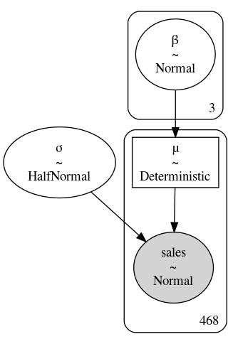
Fig. 4.19 model_pooled_sigma_sales where \(\beta\) is unpooled, as indicated by the box with 3 in the right corner, and \(\sigma\) is pooled, as the lack of number indicates a single parameter estimate for all groups. [fig:Salad_Sales_Basic_Regression_Model_Multilevel]{#fig:Salad_Sales_Basic_Regression_Model_Multilevel label=”fig:Salad_Sales_Basic_Regression_Model_Multilevel”}

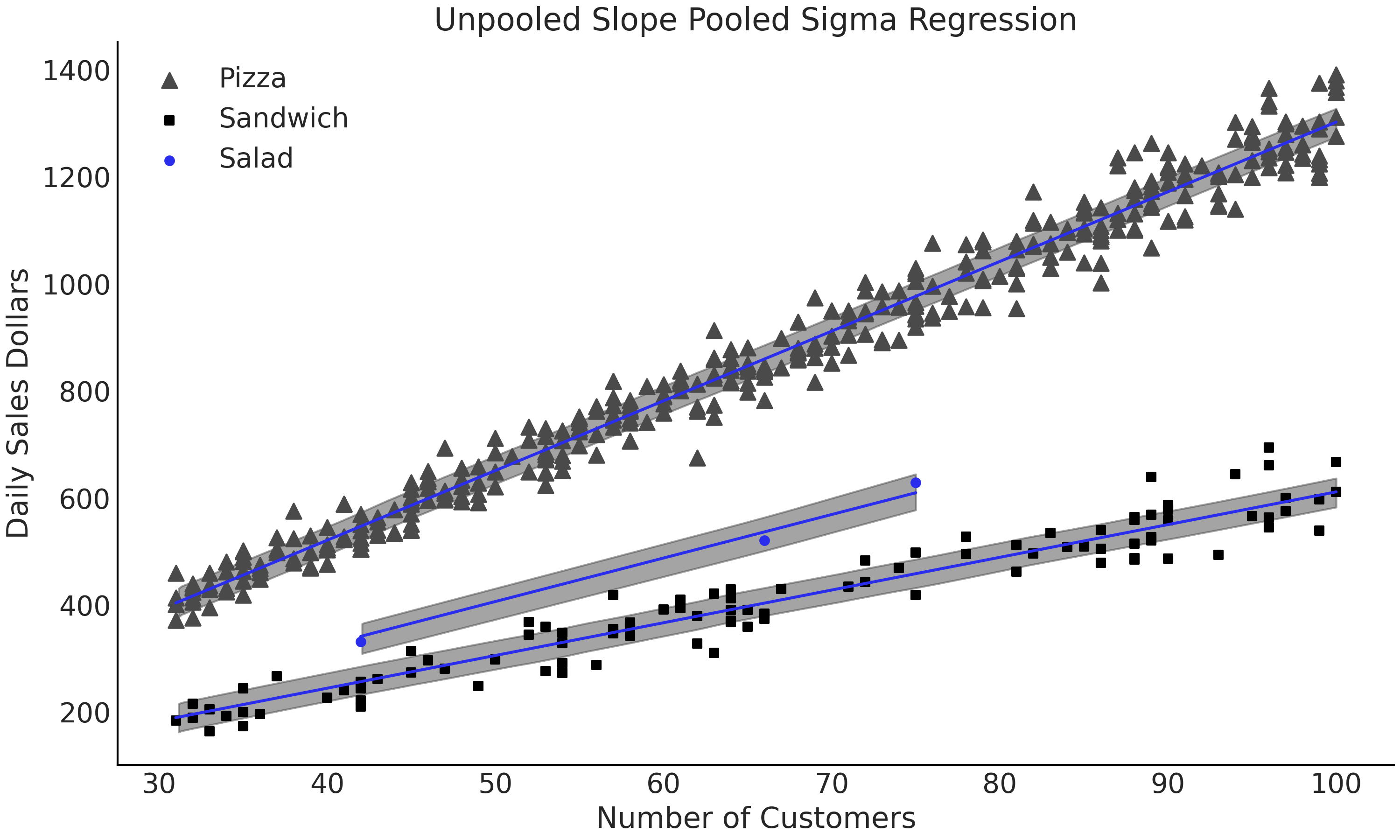
Fig. 4.20 Linear model with 50% HDI from model_pooled_sigma_sales. This model is more useful for our purposes of estimating salad sales as the slopes are independently estimated for each group. Note how all the data is being used to estimate the single posterior distribution of \(\sigma\). [fig:Salad_Sales_Basic_Regression_Scatter_Sigma_Pooled_Slope_Unpooled]{#fig:Salad_Sales_Basic_Regression_Scatter_Sigma_Pooled_Slope_Unpooled label=”fig:Salad_Sales_Basic_Regression_Scatter_Sigma_Pooled_Slope_Unpooled”}

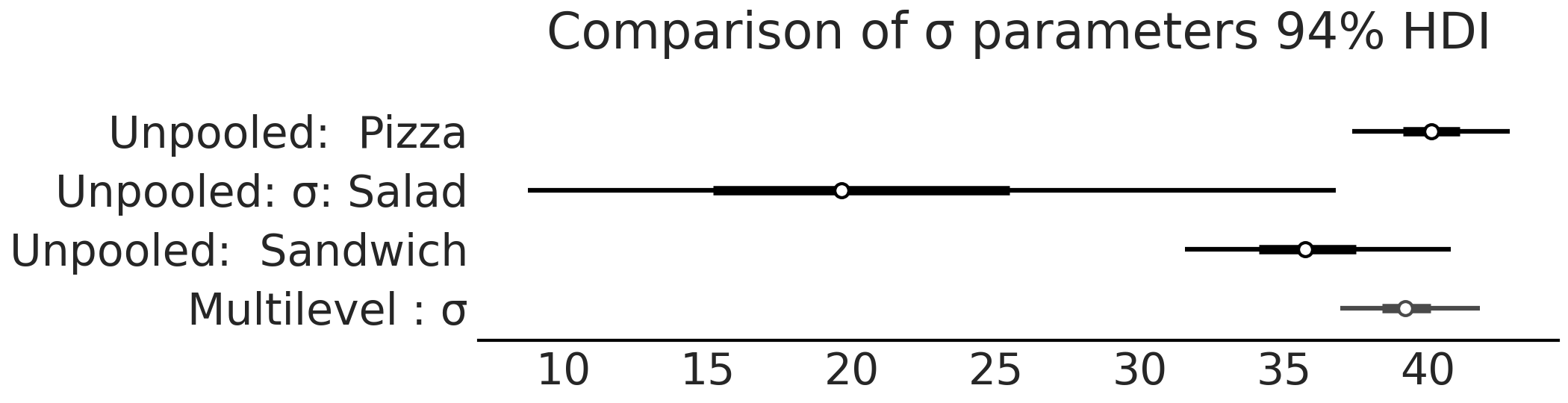
Fig. 4.21 Comparison of \(\sigma\) from model_pooled_sigma_sales and model_pooled_sales. Note how the estimated of \(\sigma\) in the multilevel model is within the bounds of the \(\sigma\) estimates from the pooled model. [fig:Salad_Sales_ForestPlot_Sigma_Unpooled_Multilevel_Comparison]{#fig:Salad_Sales_ForestPlot_Sigma_Unpooled_Multilevel_Comparison label=”fig:Salad_Sales_ForestPlot_Sigma_Unpooled_Multilevel_Comparison”}

4.6. Hierarchical Models

In our data treatment thus far we have had two options for groups, pooled where there is no distinction between groups, and unpooled where there a complete distinction between groups. Recall though in our motivating restaurant example we believed the parameter \(\sigma\) of the 3 food categories to be similar, but not exactly the same. In Bayesian modeling we can express this idea with hierarchical models. In hierarchical models the parameters are partially pooled. The partial refers to the idea that groups that do not share one fixed parameter, but share a hyperprior distribution which describes the distribution of the parameters of the prior itself. Conceptually this idea is shown in Fig. 4.22. Each group gets its own parameters which are drawn from a common hyperprior distribution.

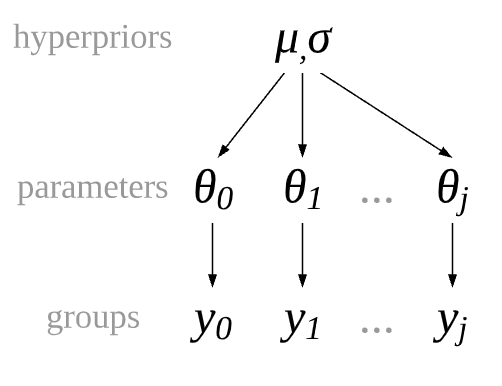
Fig. 4.22 A partially pooled model architecture where each group of observations, \(y_1, y_2, ..., y_k\) has its own set of parameters, but they are not independent as they are drawn from a common distribution.

Using statistical notation we can write a hierarchical model in Equation (4.7), the computational model in Code Block model_hierarchical_sales, and a graphical representation in Fig. 4.23.

(4.7)\[\begin{split}\begin{split} \beta_{mj} \sim& \mathcal{N}(\mu_{\beta m}, \sigma_{\beta m}) \\ \sigma_{h} \sim& \overbrace{\mathcal{HN}(\sigma)}^{\text{Hyperprior}} \\ \sigma_{j} \sim& \overbrace{\mathcal{HN}(\sigma_{h})}^{\substack{\text{Group-specific} \\ \text{pooled}}} \\ \mu_{j} =& \beta_{1j} X_1 + \dots + \beta_{mj} X_m \\ Y \sim& \mathcal{N}(\mu_{j},\sigma_{j}) \end{split}\end{split}\]

Note the addition of \(\sigma_{h}\) when compared to the multilevel model in Fig. 4.19. This is our new hyperprior distributions that defines the possible parameters of individual groups. We can add the hyperprior in Code Block model_hierarchical_sales as well. You may ask “could we have added a hyperprior for the \(\beta\) terms as well?”, and the answer is quite simply yes we could have. But in this case we assume that only the variance is related, which justifying the use of partial pooling and that the slopes are completely independent. Because this is a simulated textbook example we can plainly make this statement and “get away with it”, in a real life scenario more domain expertise and model comparison would be advised to justify this claim.

Listing 4.12 model_hierarchical_sales

with pm.Model() as model_hierarchical_sales:
    σ_hyperprior = pm.HalfNormal("σ_hyperprior", 20)
    σ = pm.HalfNormal("σ", σ_hyperprior, shape=3)
    
    β = pm.Normal("β", mu=10, sigma=20, shape=3)
    μ = pm.Deterministic("μ", β[food_category.codes] * customers)
    
    sales = pm.Normal("sales", mu=μ, sigma=σ[food_category.codes],
                      observed=sales_observed)
    
    trace_hierarchical_sales = pm.sample(target_accept=.9)
    
    inf_data_hierarchical_sales = az.from_pymc3(
        trace=trace_hierarchical_sales, 
        coords={"β_dim_0":food_category.categories,
                "σ_dim_0":food_category.categories})

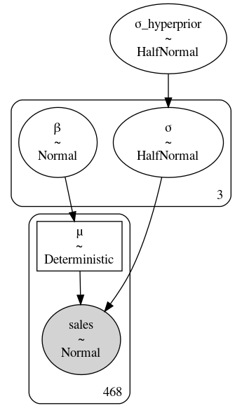
Fig. 4.23 model_hierarchical_sales where \(\sigma_{hyperprior}\) is the single hierarchical distribution for the three \(\sigma\) distributions.

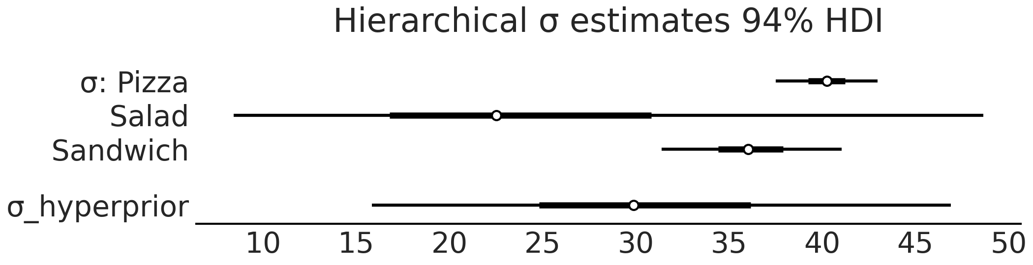
Fig. 4.24 Forest plot of the \(\sigma\) parameter estimates for model_hierarchical_sales. Note how the hyperprior tends to represent fall within the range of the three group priors.

After fitting the hierarchical model we can inspect the \(\sigma\) parameter estimates in Fig. 4.24. Again note the addition of \(\sigma_{hyperprior}\) which is a distribution that estimates the distribution of the parameters for each of the three food categories. We can also see the effect of a hierarchical model if we compare the summary tables of the unpooled model and hierarchical models in Table 4.3. In the unpooled estimate the mean of the \(\sigma\) estimate for salads is 21.3, whereas in the hierarchical estimate the mean of the same parameter estimate is now 25.5, and has been “pulled” up by the means of the pizza and sandwiches category. Moreover, the estimates of the pizza and sandwich categories in the hierarchical category, while regressed towards the mean slightly, remain largely the same as the unpooled estimates. Note how the estimates of each sigma are distinctly different from each other. Given that our observed data and the model which does not share information between groups this consistent with our expectations.

Table 4.3 Estimates of σ for each category from the unpooled sales model

	mean	sd	hdi_3%	hdi_97%
\(\sigma\)Pizza	40.1	1.5	37.4	42.8
\(\sigma\)Salad	21.3	8.3	8.8	36.8
\(\sigma\)Sandwich	35.9	2.5	31.6	40.8

Table 4.4 Estimates of σ for each category from the hierarchical sales model

	mean	sd	hdi_3%	hdi_97%
\(\sigma\)Pizza	40.3	1.5	37.5	43.0
\(\sigma\)Salad	25.5	12.4	8.4	48.7
\(\sigma\)Sandwich	36.2	2.6	31.4	41.0
\(\sigma_{hyperprior}\)	31.2	8.7	15.8	46.9

I heard you like hyperpriors so I put a hyperpriors on top of your hyperpriors

In Code Block model_hierarchical_salad_sales_centered we placed hyperprior on group level parameter \(\sigma_j\). Similarly, we can extend the model by also adding hyperprior to parameter \(\beta_{mj}\). Note that since \(\beta_{mj}\) has a Gaussian distributed prior, we can actually choose two hyperprior - one for each hyperparameter. A natural question you might ask is can we go even further and adding hyperhyperprior to the parameters that are parameterized the hyperprior? What about hyperhyperhyperprior? While it is certainly possible to write down such models and sample from it, it is worth to take a step back and think about what hyperpriors are doing. Intuitively, they are a way for the model to “borrow” information from sub-group or sub-cluster of data to inform the estimation of other sub-group/cluster with less observation. The group with more observations will inform the posterior of the hyperparameter, which then in turn regulates the parameters for the group with less observations. In this lens, putting hyperprior on parameters that are not group specific is quite meaningless.

Hierarchical estimates are not just limited to two levels. For example, the restaurant sales model could be extended into a three-level hierarchical model where the top level represented the company level, the next level represented the geographical market (New York, Chicago, Los Angeles), and the lowest level represented an individual location. By doing so we can have a hyperprior characterizing how the whole company was doing, hyperpriors indicating how a region was doing, and priors on how each store was doing. This allows easy comparisons in mean and variation, and expands the application in many different ways based on a single model.

4.6.1. Posterior Geometry Matters

So far we have largely focused on the structure and math behind the model, and assumed our sampler would be able to provide us an “accurate” estimate of the posterior. And for relatively simple models this is largely true, the newest versions of Universal Inference Engines mostly “just work”, but an important point is that they do not always work. Certain posterior geometries are challenging for samplers, a common example is Neal’s Funnel[45] shown in Fig. 4.25. As the name funnel connotes, the shape at one end is quite wide, before narrowing into a small neck. Recalling Section A DIY Sampler, Do Not Try This at Home samplers function by taking steps from one set of parameter values to another, and a key setting is how big of a step to take when exploring the posterior surface. In complex geometries, such as with Neal’s funnel, a step size that works well in one area, fails miserably in another.

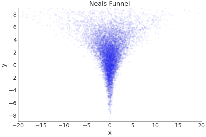
Fig. 4.25 Correlated samples in a particular shape referred to as Neal’s Funnel. At sampling at the top of the funnel where Y is around a value 6 to 8, a sampler can take wide steps of lets say 1 unit, and likely remain within a dense region of the posterior. However, if sampling near the bottom of the funnel where Y is around a value -6 to -8, a 1 unit step in almost any direction will likely result in step into a low-density region. This drastic difference in the posterior geometry shape is one reason poor posterior estimation, can occur for sampling based estimates. For HMC samplers the occurence of divergences can help diagnose these sampling issues.

In hierarchical models the geometry is largely defined by the correlation of hyperpriors to other parameters, which can result in funnel geometry that are difficult to sample. Unfortunately this is not only a theoretical problem, but a practical one, that can sneak up relatively quickly on an unsuspecting Bayesian modeler. Luckily, there is a relatively easy tweak to models, referred to as a non-centered parameterization, that helps alleviate the issue.

Continuing with our salad example, let us say we open 6 salad restaurants and like before are interested in predicting the sales as a function of the number of customers. The synthetic dataset has been generated in Python and is shown in Fig. 4.26. Since the restaurants are selling the exact same product a hierarchical model is appropriate to share information across groups. We write the centered model mathematically in Equation (4.8) and also Code Block model_hierarchical_salad_sales. We will be using TFP and tfd.JointDistributionCoroutine in the rest of the chapter, which more easily highlights the change in parameterization. This model follows the standard hierarchical format, where a hyperprior partially pools the parameters of the slope \(\beta_m\).

(4.8)\[\begin{split}\begin{split} \beta_{\mu h} \sim& \mathcal{N} \\ \beta_{\sigma h} \sim& \mathcal{HN} \\ \beta_m \sim& \overbrace{\mathcal{N}(\beta_{\mu h},\beta_{\sigma h})}^{\text{Centered}} \\ \sigma_{h} \sim& \mathcal{HN} \\ \sigma_{m} \sim& \mathcal{HN}(\sigma_{h}) \\ Y \sim& \mathcal{N}(\beta_{m} * X_m,\sigma_{m}) \end{split}\end{split}\]

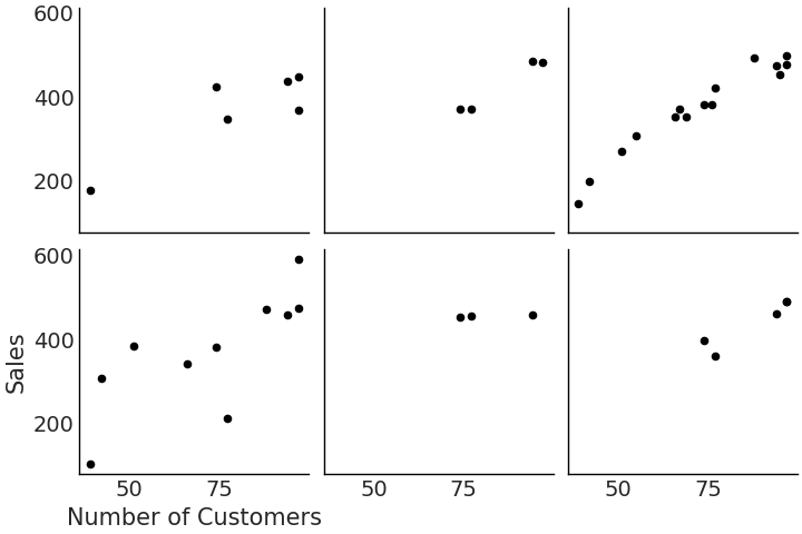
Fig. 4.26 Observed salad sales across 6 locations. Note how some locations have very few data points relative to others.

Listing 4.13 model_hierarchical_salad_sales

def gen_hierarchical_salad_sales(input_df, beta_prior_fn, dtype=tf.float32):
    customers = tf.constant(input_df["customers"].values, dtype=dtype)
    location_category = input_df["location"].values
    sales = tf.constant(input_df["sales"].values, dtype=dtype)

    @tfd.JointDistributionCoroutine
    def model_hierarchical_salad_sales():
        β_μ_hyperprior = yield root(tfd.Normal(0, 10, name="beta_mu"))
        β_σ_hyperprior = yield root(tfd.HalfNormal(.1, name="beta_sigma"))
        β = yield from beta_prior_fn(β_μ_hyperprior, β_σ_hyperprior)

        σ_hyperprior = yield root(tfd.HalfNormal(30, name="sigma_prior"))
        σ = yield tfd.Sample(tfd.HalfNormal(σ_hyperprior), 6, name="sigma")

        loc = tf.gather(β, location_category, axis=-1) * customers
        scale = tf.gather(σ, location_category, axis=-1)
        sales = yield tfd.Independent(tfd.Normal(loc, scale),
                                      reinterpreted_batch_ndims=1,
                                      name="sales")

    return model_hierarchical_salad_sales, sales

Similar to the TFP models we used in Chapter 3, the model is wrapped within a function so we can condition on an arbitrary inputs more easily. Besides the input data, gen_hierarchical_salad_sales also takes a callable beta_prior_fn which defines the prior of slope \(\beta_m\). Inside the Coroutine model we use a yield from statement to invoke the beta_prior_fn. This description may be too abstract in words but is easier to see action in Code Block model_hierarchical_salad_sales_centered:

Listing 4.14 model_hierarchical_salad_sales_centered

def centered_beta_prior_fn(hyper_mu, hyper_sigma):
    β = yield tfd.Sample(tfd.Normal(hyper_mu, hyper_sigma), 6, name="beta")
    return β

# hierarchical_salad_df is the generated dataset as pandas.DataFrame
centered_model, observed = gen_hierarchical_salad_sales(
    hierarchical_salad_df, centered_beta_prior_fn)

As shown above, Code Block model_hierarchical_salad_sales_centered defined a centered parameterization of the slope \(\beta_m\), which follows a Normal distribution with hyper_mu and hyper_sigma. centered_beta_prior_fn is a function that yields a tfp.distribution, similar to the way we write a tfd.JointDistributionCoroutine model. Now that we have our model, we can run inference and inspect the result in Code Block model_hierarchical_salad_sales_centered_inference.

Listing 4.15 model_hierarchical_salad_sales_centered_inference

mcmc_samples_centered, sampler_stats_centered = run_mcmc(
    1000, centered_model, n_chains=4, num_adaptation_steps=1000,
    sales=observed)

divergent_per_chain = np.sum(sampler_stats_centered["diverging"], axis=0)
print(f"""There were {divergent_per_chain} divergences after tuning per chain.""")

There were [37 31 17 37] divergences after tuning per chain.

We reuse the inference code previously shown in Code Block tfp_posterior_inference to run our model. After running our model the first indication of issues is the divergences, the details of which we covered in Section Divergences. A plot of the sample space is the next diagnostic and is shown in Fig. 4.27. Note how as the hyperprior \(\beta_{\sigma h}\) approaches zero, the width of the posterior estimate of the \(\beta_m\) parameters tend to shrink. In particular note how there are no samples near zero. In other words as the value \(\beta_{\sigma h}\) approaches zero, there the region in which to sample parameter \(\beta_m\) collapses and the sampler is not able to effectively characterize this space of the posterior.

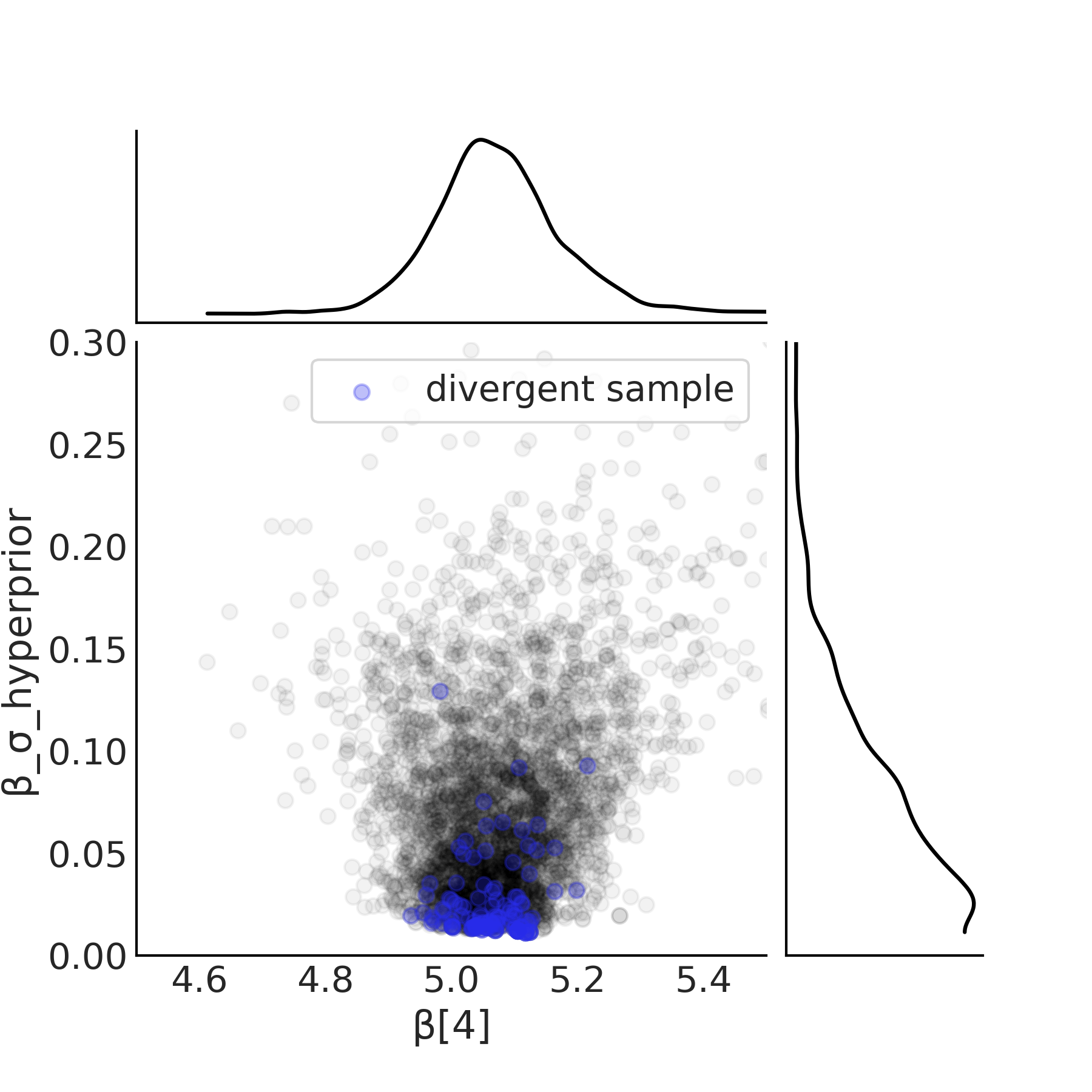
Fig. 4.27 Scatter plot of the hyperprior and the slope of \(\beta[4]\) from centered_model defined in Code Block model_hierarchical_salad_sales_centered. As the hyperprior approaches zero the posterior space for slope collapses results in the divergences seen in blue.

To alleviate this issue the centered parameterization can be converted into a non-centered parameterization shown in Code Block in model_hierarchical_salad_sales_non_centered and Equation (4.9). The key difference is that instead of estimating parameters of the slope \(\beta_m\) directly, it is instead modeled as a common term shared between all groups and a term for each group that captures the deviation from the common term. This modifies the posterior geometry in a manner that allows the sampler to more easily explore all possible values of \(\beta_{\sigma h}\). The effect of this posterior geometry change is as shown in Fig. 4.28, where there are multiple samples down to the 0 value on the x-axis.

(4.9)\[\begin{split}\begin{split} \beta_{\mu h} \sim& \mathcal{N} \\ \beta_{\sigma h} \sim& \mathcal{HN} \\ \beta_\text{m_offset} \sim& \mathcal{N}(0,1) \\ \beta_m =& \overbrace{\beta_{\mu h} + \beta_\text{m_offset}*\beta_{\sigma h}}^{\text{Non-centered}} \\ \sigma_{h} \sim& \mathcal{HN} \\ \sigma_{m} \sim& \mathcal{HN}(\sigma_{h}) \\ Y \sim& \mathcal{N}(\beta_{m} * X_m,\sigma_{m}) \end{split}\end{split}\]

Listing 4.16 model_hierarchical_salad_sales_non_centered

def non_centered_beta_prior_fn(hyper_mu, hyper_sigma):
    β_offset = yield root(tfd.Sample(tfd.Normal(0, 1), 6, name="beta_offset"))
    return β_offset * hyper_sigma[..., None] + hyper_mu[..., None]

# hierarchical_salad_df is the generated dataset as pandas.DataFrame
non_centered_model, observed = gen_hierarchical_salad_sales(
    hierarchical_salad_df, non_centered_beta_prior_fn)

mcmc_samples_noncentered, sampler_stats_noncentered = run_mcmc(
    1000, non_centered_model, n_chains=4, num_adaptation_steps=1000,
    sales=observed)

divergent_per_chain = np.sum(sampler_stats_noncentered["diverging"], axis=0)
print(f"There were {divergent_per_chain} divergences after tuning per chain.")

There were [1 0 2 0] divergences after tuning per chain.

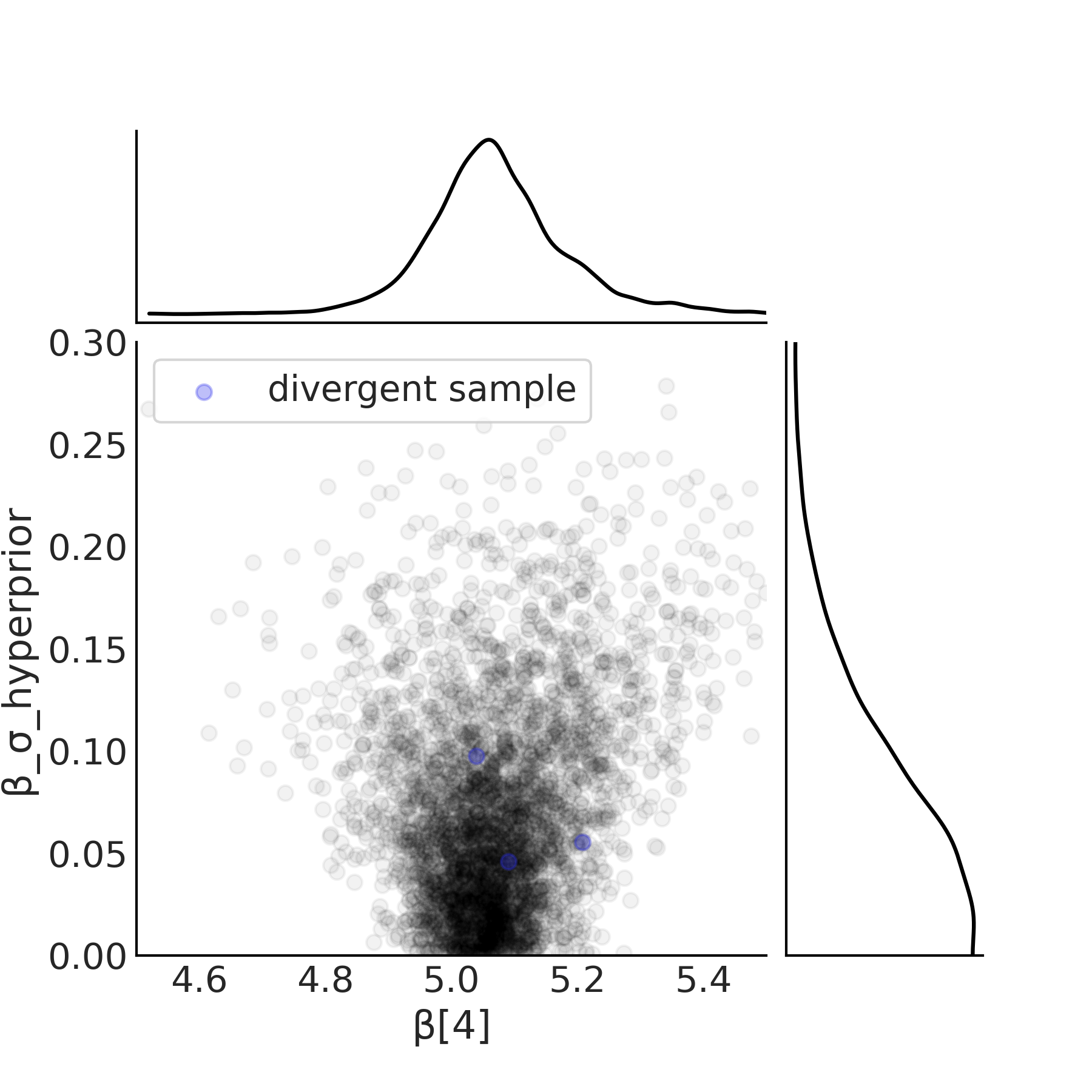
Fig. 4.28 Scatter plot of the hyperprior and the estimated slope \(\beta[4]\) of location 4 from non_centered_model defined in Code Block model_hierarchical_salad_sales_non_centered. In the non-centered parameterization the sampler is able to sample parameters close to zero. The divergences are lesser in number and are not concentrated in one area.

The improvement in sampling has a material effect on the estimated distribution shown in Fig. 4.29. While it may be jarring to be reminded of this fact again, samplers merely estimate the posterior distribution, and while in many cases they do quite well, it is not guaranteed! Be sure to pay heed to the diagnostics and investigate more deeply if warnings arise.

It is worth noting that there is no one size fits all solution when it comes to centered or non-centered parameterization [46]. It is a complex interaction among the informativeness of the individual likelihood at group level (usually the more data you have for a specific group, the more informative the likelihood function will be), the informativeness of the group level prior, and the parameterization. A general heuristic is that if there are not a lot of observations, a non-centered parameterization is preferred. In practice however, you should try a few different combinations of centered and non-centered parameterizations, with different prior specifications. You might even find cases where you need both centered and non-centered parameterization in a single model. We recommend you to read Michael Betancourt’s case study Hierarchical Modeling on this topic if you suspect model parameterization is causing you sampling issues [47].

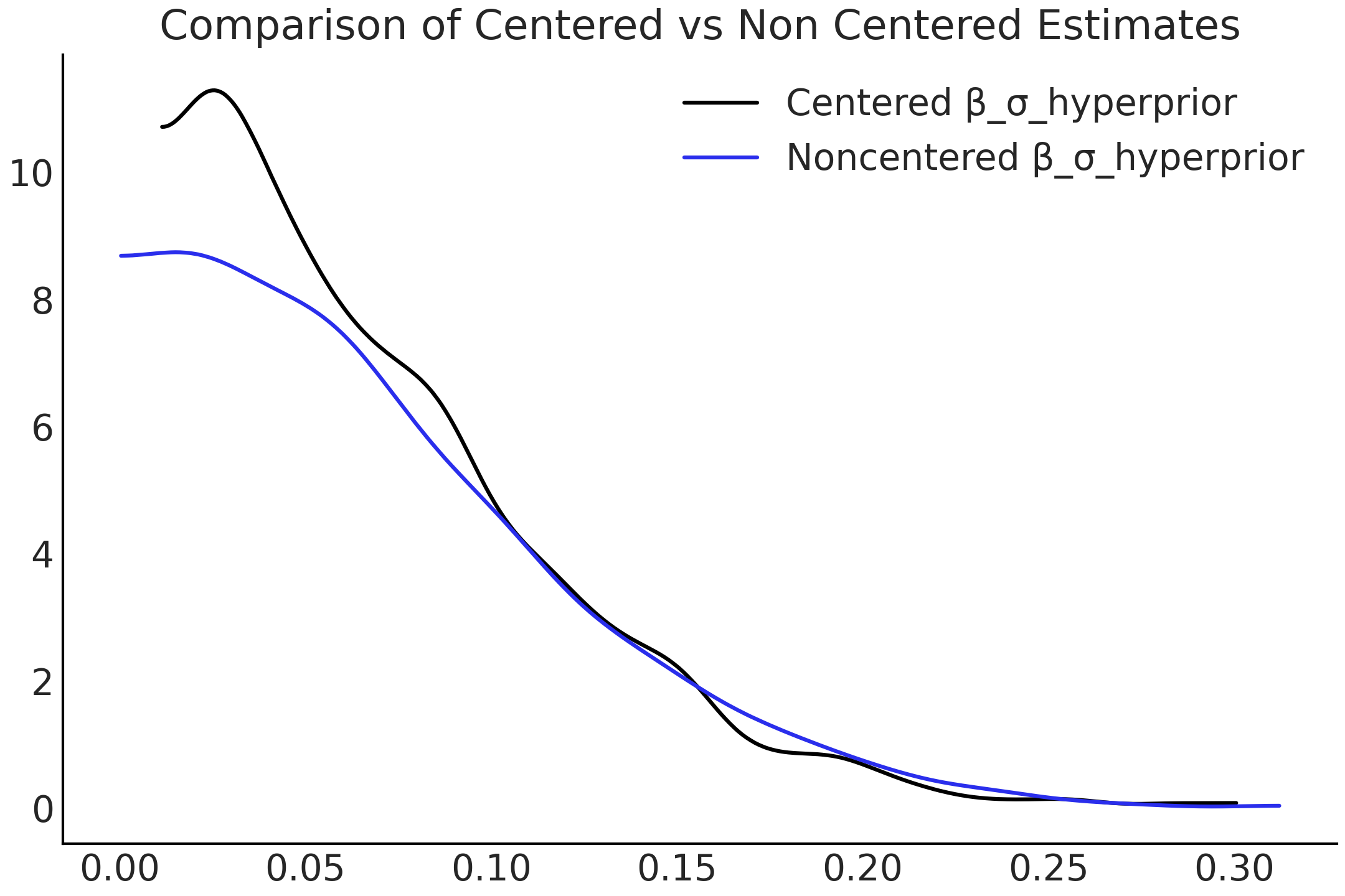
Fig. 4.29 KDE of the distributions of \(\beta_{\sigma h}\) in both centered and non-centered parameterizations. The change is due to the sampler being able to more adequately explore the possible parameter space.

4.6.2. Predictions at Multiple Levels

A subtle feature of hierarchical models is that they are able to make estimates at multiple levels. While seemingly obvious this is very useful, as it lets us use one model to answer many more questions than a single level model. In Chapter 3 we could built a model to estimate the mass of a single species or a separate model to estimate the mass of any penguin regardless of species. Using a hierarchical model we could estimate the mass of all penguins, and each penguin species, at the same time with one model. With our salad sales model we can both make estimations about an individual location and about the population a whole. We can do so by using our previous non_centered_model from Code Block model_hierarchical_salad_sales_non_centered, and write an out_of_sample_prediction_model as shown in Code Block model_hierarchical_salad_sales_predictions. This using the fitted parameter estimates to make an out of sample prediction for the distribution of customers for 50 customers, at two locations and for the company as a whole simultaneously. Since our non_centered_model is also a TFP distribution, we can nest it into another tfd.JointDistribution, doing so constructed a larger Bayesian graphical model that extends our initial non_centered_model to include nodes for out of sample prediction. The estimates are plotted in Fig. 4.30.

Listing 4.17 model_hierarchical_salad_sales_predictions

out_of_sample_customers = 50.

@tfd.JointDistributionCoroutine
def out_of_sample_prediction_model():
    model = yield root(non_centered_model)
    β = model.beta_offset * model.beta_sigma[..., None] + model.beta_mu[..., None]
    
    β_group = yield tfd.Normal(
        model.beta_mu, model.beta_sigma, name="group_beta_prediction")
    group_level_prediction = yield tfd.Normal(
        β_group * out_of_sample_customers,
        model.sigma_prior,
        name="group_level_prediction")
    for l in [2, 4]:
        yield tfd.Normal(
            tf.gather(β, l, axis=-1) * out_of_sample_customers,
            tf.gather(model.sigma, l, axis=-1),
            name=f"location_{l}_prediction")

amended_posterior = tf.nest.pack_sequence_as(
    non_centered_model.sample(),
    list(mcmc_samples_noncentered) + [observed])

ppc = out_of_sample_prediction_model.sample(var0=amended_posterior)

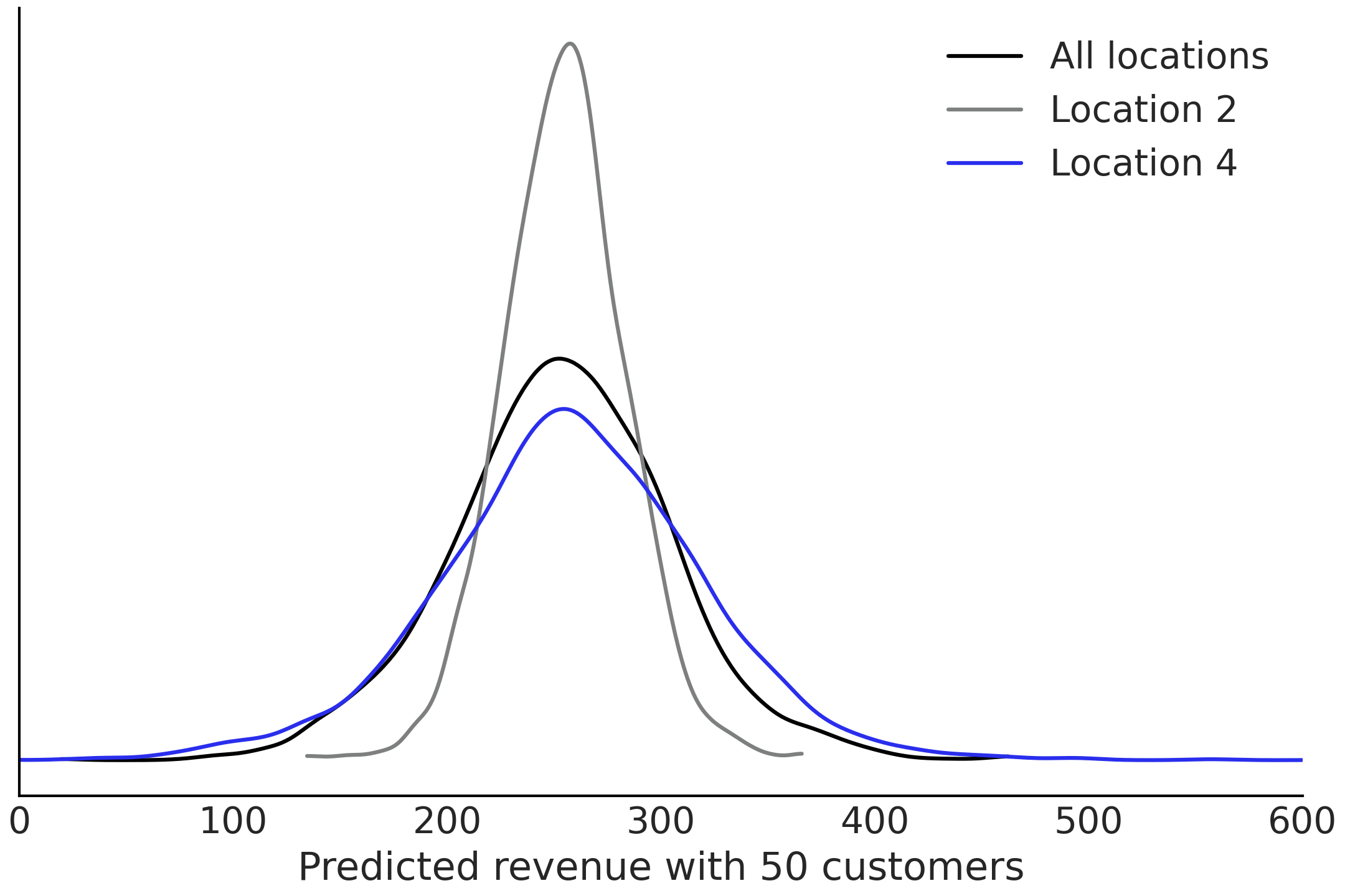
Fig. 4.30 Posterior predictive estimates for the revenues for two of the groups and for total population estimated by model model_hierarchical_salad_sales_non_centered.

Another feature in making predictions is using hierarchical models with hyperpriors is that we can make prediction for never before seen groups. In this case, imagine we are opening another salad restaurant in a new location we can already make some predictions of how the salad sales might looks like by first sampling from the hyper prior to get the \(\beta_{i+1}\) and \(\sigma_{i+1}\) of the new location, then sample from the posterior predictive distribution to get salad sales prediction. This is demonstrated in Code Block model_hierarchical_salad_sales_predictions_new_location.

Listing 4.18 model_hierarchical_salad_sales_predictions_new_location

out_of_sample_customers2 = np.arange(50, 90)

@tfd.JointDistributionCoroutine
def out_of_sample_prediction_model2():
    model = yield root(non_centered_model)
    
    β_new_loc = yield tfd.Normal(
        model.beta_mu, model.beta_sigma, name="beta_new_loc")
    σ_new_loc = yield tfd.HalfNormal(model.sigma_prior, name="sigma_new_loc")
    group_level_prediction = yield tfd.Normal(
        β_new_loc[..., None] * out_of_sample_customers2,
        σ_new_loc[..., None],
        name="new_location_prediction")

ppc = out_of_sample_prediction_model2.sample(var0=amended_posterior)

In addition to the mathematical benefits of hierarchical modeling, there is a benefit from a computational perspective as we only need to construct and fit a single model. This speeds up the modeling process and the subsequent model maintenance process, if the model is reused multiple times over time.

On the validity of LOO

Hierarchical models allow us to make posterior predictions even for group(s) that have never been seen before. However, how valid would the prediction be? Could we use cross-validation to assess the performance of the model? As usually in statistics the answer is that depends. Whether cross-validation (and methods like LOO and WAIC) is valid or not depends on the prediction task you want to perform, and also on the data generating mechanism. If we want to use LOO to assess how well the model is able to predict new observations , then LOO is fine. Now if we want to assess how well one entire group is predicted, then you will need to perform leave one-group-out cross validation, which is a well defined procedure. In that case however, the LOO method will most likely not be good, as we are removing many observations at a time and the importance sampling step at the core of the LOO approximation relies on the distributions with and without the point/group/etc being close to each other.

4.6.3. Priors for Multilevel Models

Prior choice is all the more important for multilevel models, because of how the prior interacts with the informativeness of the likelihood, as shown above in Section Posterior Geometry Matters. Moreover, not only does the shape of prior distribution matter, we also have additional choices of how to parameterize them. This does not limit us to Gaussian priors as it applies to all distributions in the location-scale distribution family [6].

In multilevel models prior distributions not only characterize the in-group variation, but the between-group variation as well. In a sense the choice of hyperprior is defining the “variation of variation”, which could make expressing and reasoning about prior information difficult. Moreover, since the effect of partial pooling is the combination of how informative the hyperprior is, the number of groups you have, and the number of observations in each group. Due to this the same hyperprior might not work if you are performing inference using the same model on similar dataset but with fewer groups.

As is such besides empirical experience (e.g., general recommendations published in articles) or general advice [7], we can also perform sensitivity studies to better inform our prior choice. For instance Lemoine [48] showed that when modeling ecology data with a model structure of

(4.10)\[\begin{split}\begin{split} \alpha_i \sim& \mathcal{N}(\mu_{\alpha},\sigma^2_{\alpha}) \\ \mu_{i} =& \alpha_i + \beta Day_i \\ Y \sim& \mathcal{N}(\mu_{j},\sigma^2) \end{split}\end{split}\]

where the intercept is unpooled, Cauchy priors provide regularization at few data points, and do not obscure the posterior when the model is fitted on additional data. This is done through prior sensitivity analysis across both prior parameterizations and differing amounts of data. In your own multilevel models be sure to note multitude of ways a prior choice affects inference, and use either your domain expertise or tools such as prior predictive distributions to make an informed choice.

4.7. Exercises

4E1. What are examples of covariate-response relationships that are nonlinear in everyday life?

4E2. Assume you are studying the relationship between a covariate and an outcome and the data can be into 2 groups. You will be using a regression with a slope and intercept as your basic model structure.

\[\begin{split}\begin{split} \mu =& \beta_0 + \beta_1 X_1 \\ Y \sim& \mathcal{N}(\mu, \sigma) \end{split}\end{split}\]

Also assume you now need to extend the model structure in each of the ways listed below. For each item write the mathematical equations that specify the full model.

1. Pooled

2. Unpooled

3. Mixed Effect with pooled \(\beta_0\)

4. Hierarchical \(\beta_0\)

5. Hierarchical all parameters

6. Hierarchical all parameters with non-centered \(\beta\) parameters

4E3. Use statistical notation to write a robust linear regression model for the baby dataset.

4E4. Consider the plight of a bodybuilder who needs to lift weights, do cardiovascular exercise, and eat to build a physique that earns a high score at a contest. If we were to build a model where weightlifting, cardiovascular exercise, and eating were covariates do you think these covariates are independent or do they interact? From your domain knowledge justify your answer?

4E5. An interesting property of the Student’s t-distribution is that at values of \(\nu = 1\) and \(\nu = \infty\), the Student’s t-distribution becomes identical two other distributions the Cauchy distribution and the Normal distribution. Plot the Student’s t-distribution at both parameter values of \(\nu\) and match each parameterization to Cauchy or Normal.

4E6. Assume we are trying to predict the heights of individuals. If given a dataset of height and one of the following covariates explain which type of regression would be appropriate between unpooled, pooled, partially pooled, and interaction. Explain why

1. A vector of random noise

2. Gender

3. Familial relationship

4. Weight

4E7. Use LOO to compare the results of baby_model_linear and baby_model_sqrt. Using LOO justify why the transformed covariate is justified as a modeling choice.

4E8. Go back to the penguin dataset. Add an interaction term to estimate penguin mass between species and flipper length. How do the predictions differ? Is this model better? Justify your reasoning in words and using LOO.

4M9. Ancombe’s Quartet is a famous dataset highlighting the challenges with evaluating regressions solely on numerical summaries. The dataset is available at the GitHub repository. Perform a regression on the third case of Anscombe’s quartet with both robust and non-robust regression. Plot the results.

4M10. Revisit the penguin mass model defined in Code Block nocovariate_mass. Add a hierarchical term for \(\mu\). What is the estimated mean of the hyperprior? What is the average mass for all penguins? Compare the empirical mean to the estimated mean of the hyperprior. Do the values of the two estimates make sense to you, particularly when compared to each other? Why?

4M11. The compressive strength of concrete is dependent on the amount of water and cement used to produce it. In the GitHub repository we have provided a dataset of concrete compressive strength, as well the amount of water and cement included (kilograms per cubic meter). Create a linear model with an interaction term between water and cement. What is different about the inputs of this interaction model versus the smoker model we saw earlier? Plot the concrete compressive strength as function of concrete at various fixed values of water.

4M12. Rerun the pizza regression but this time do it with heteroskedastic regression. What are the results?

4H13. Radon is a radioactive gas that can cause lung cancer and thus it is something that would be undesirable in a domicile. Unfortunately the presence of a basement may increase the radon levels in a household as radon may enter the household more easily through the ground. We have provided a dataset of the radon levels at homes in Minnesota, in the GitHub repository as well as the county of the home, and the presence of a basement.

1. Run an unpooled regression estimating the effect of basements on radon levels.

2. Create a hierarchical model grouping by county. Justify why this model would be useful for the given the data.

3. Create a non-centered regression. Using plots and diagnostics justify if the non-centered parameterization was needed.

4H14. Generate a synthetic dataset for each of the models below with your own choice of parameters. Then fit two models to each dataset, one model matching the data generating process, and one that does not. See how the diagnostic summaries and plots differ between the two.

For example, we may generate data that follows a linear pattern \(x=[1,2,3,4], y=[2,4,6,8]\). Then fit a model of the form \(y=bx\) and another of the form \(y=bx**2\)

1. Linear Model

2. Linear model with transformed covariate

3. Linear model with interaction effect

4. 4 group model with pooled intercept, and unpooled slope and noise

5. A Hierarchical Model

4H15. For the hierarchical salad regression model evaluate the posterior geometry for the slope parameter \(\beta_{\mu h}\). Then create a version of the model where \(\beta_{\mu h}\) is non-centered. Plot the geometry now. Are there any differences? Evaluate the divergences and output as well. Does non-centering help in this case?

4H16. A colleague of yours, who now lives on an unknown planet, ran experiment to test the basic laws of physics. She dropped a ball of a cliff and registers the position for 20 seconds. The data is available in the Github repository in the file gravity_measurements.csv You know that from Newton’s Laws of physics if the acceleration is \(g\) and the time \(t\) then

(4.11)\[\begin{split}\begin{split} \text{velocity} &= gt \\ \text{position} &= \frac{1}{2}gt^2 \\ \end{split}\end{split}\]

Your friend asks you to estimate the following quantities

1. The gravitational constant of the planet

2. A characterization of the noise of her measurement device

3. The velocity of the ball at each point during her measurements

4. The estimated position of the ball from time 20 to time 30

---

[1]

The difference between the observed value and the estimated value of a quantity of interest is call the residual.

[2]

Remember this is just a toy dataset, so the take-home message should be about modeling interactions and not about tips.

[3]

Although the mean is defined only for \(\nu > 1\), and the value of \(\sigma\) agrees with the standard deviation only when \(\nu \to \infty\).

[4]

A thin dough filled with a salty or sweet preparation and baked or fried. The filling can include red or white meat, fish, vegetables, or fruit. Empanadas are common in Southern European, Latin American, and the Filipino cultures.

[5]

The commemoration of the first Argentine government and the Argentine independence day respectively.

[6]

https://en.wikipedia.org/wiki/Location–scale_family

[7]

stan-dev/stan