Code 6: Time Series

This is a reference notebook for the book Bayesian Modeling and Computation in Python

The textbook is not needed to use or run this code, though the context and explanation is missing from this notebook.

If you’d like a copy it’s available from the CRC Press or from Amazon. ``

import matplotlib.pyplot as plt
import arviz as az
import pandas as pd
import numpy as np

import tensorflow as tf
import tensorflow_probability as tfp

tfd = tfp.distributions
tfb = tfp.bijectors
root = tfd.JointDistributionCoroutine.Root

import datetime
print(f"Last Run {datetime.datetime.now()}")

az.style.use("arviz-grayscale")
plt.rcParams["figure.dpi"] = 300

Time Series Analysis as a Regression Problem

Code 6.1

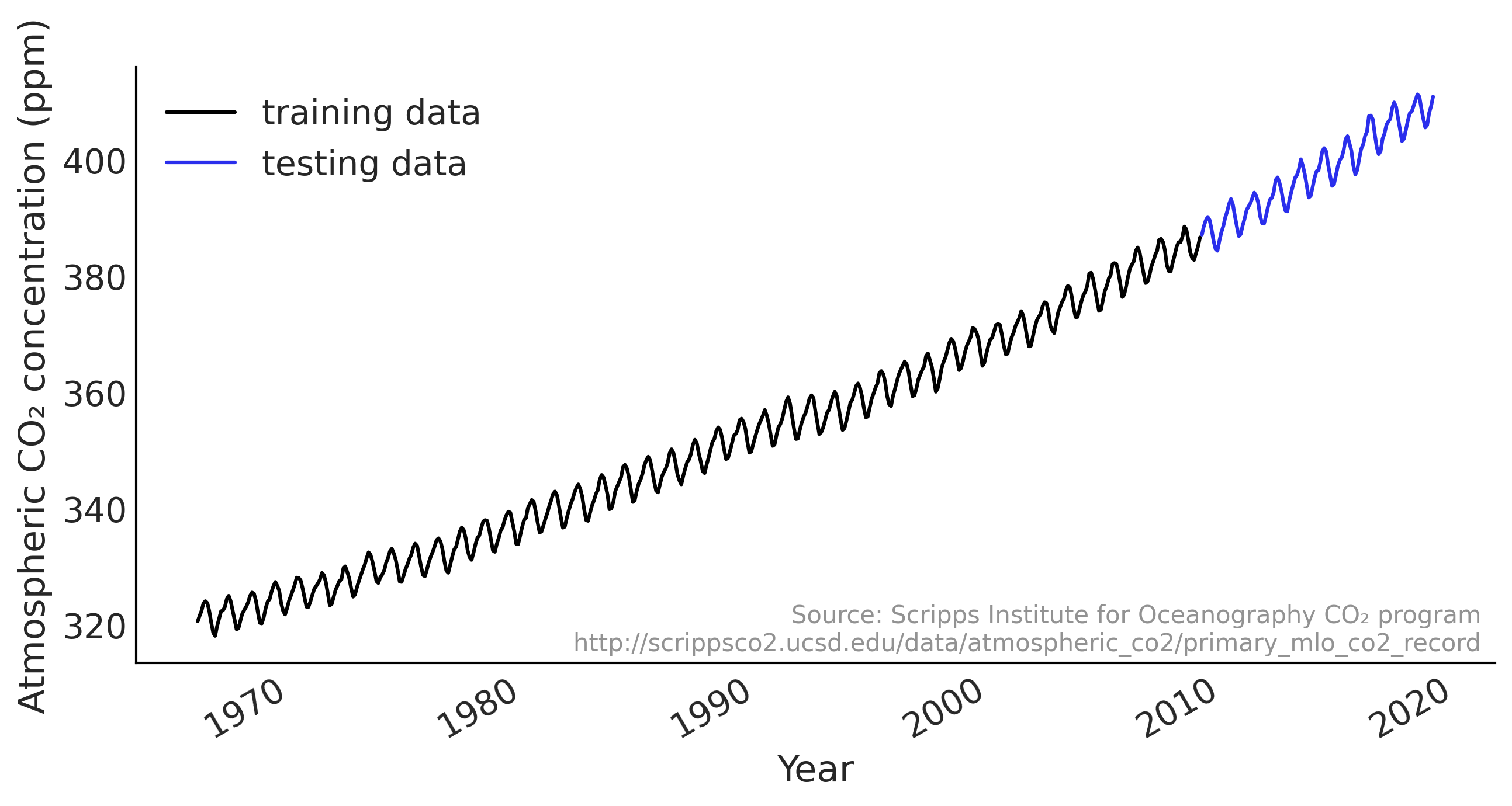
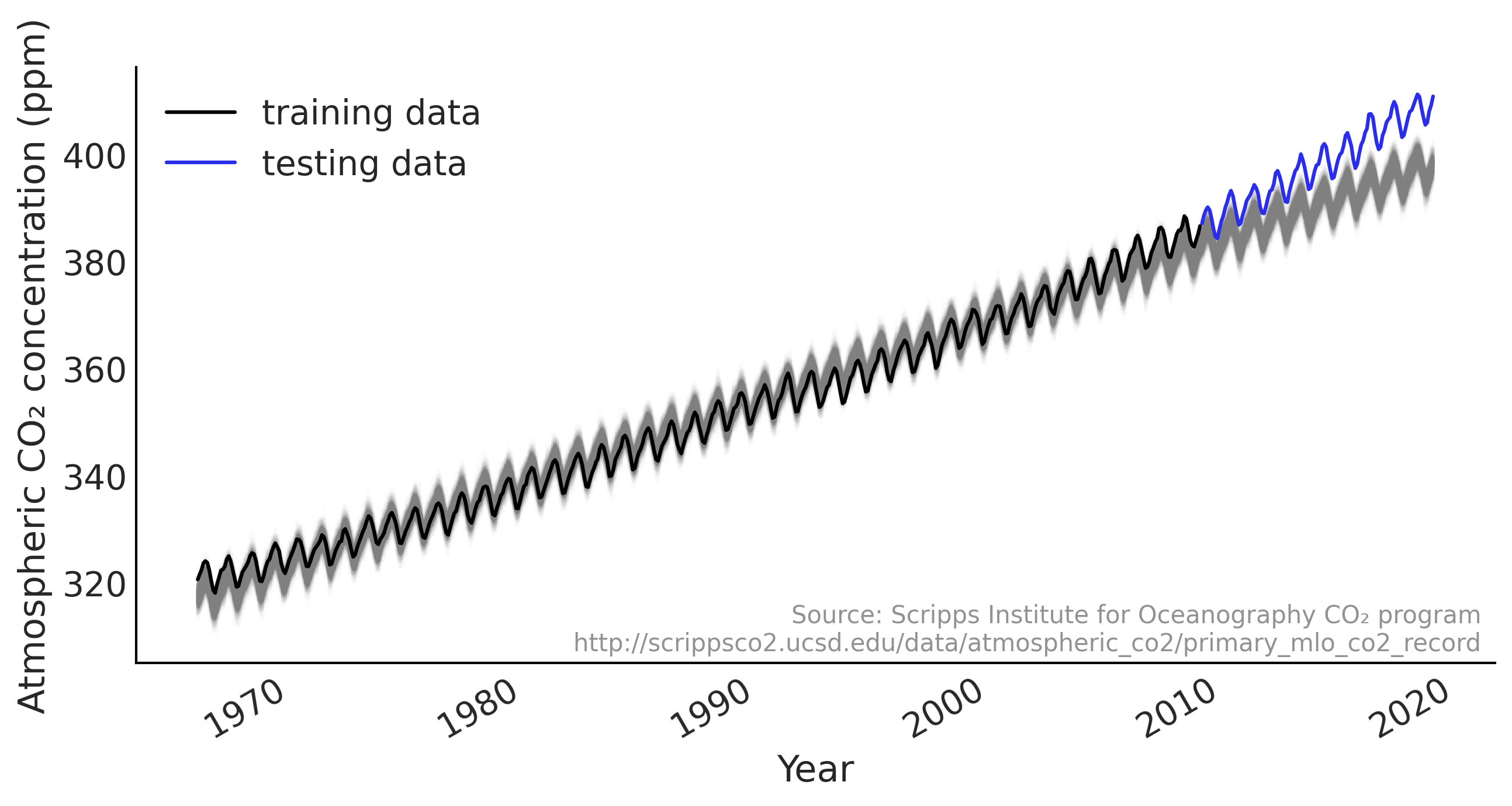
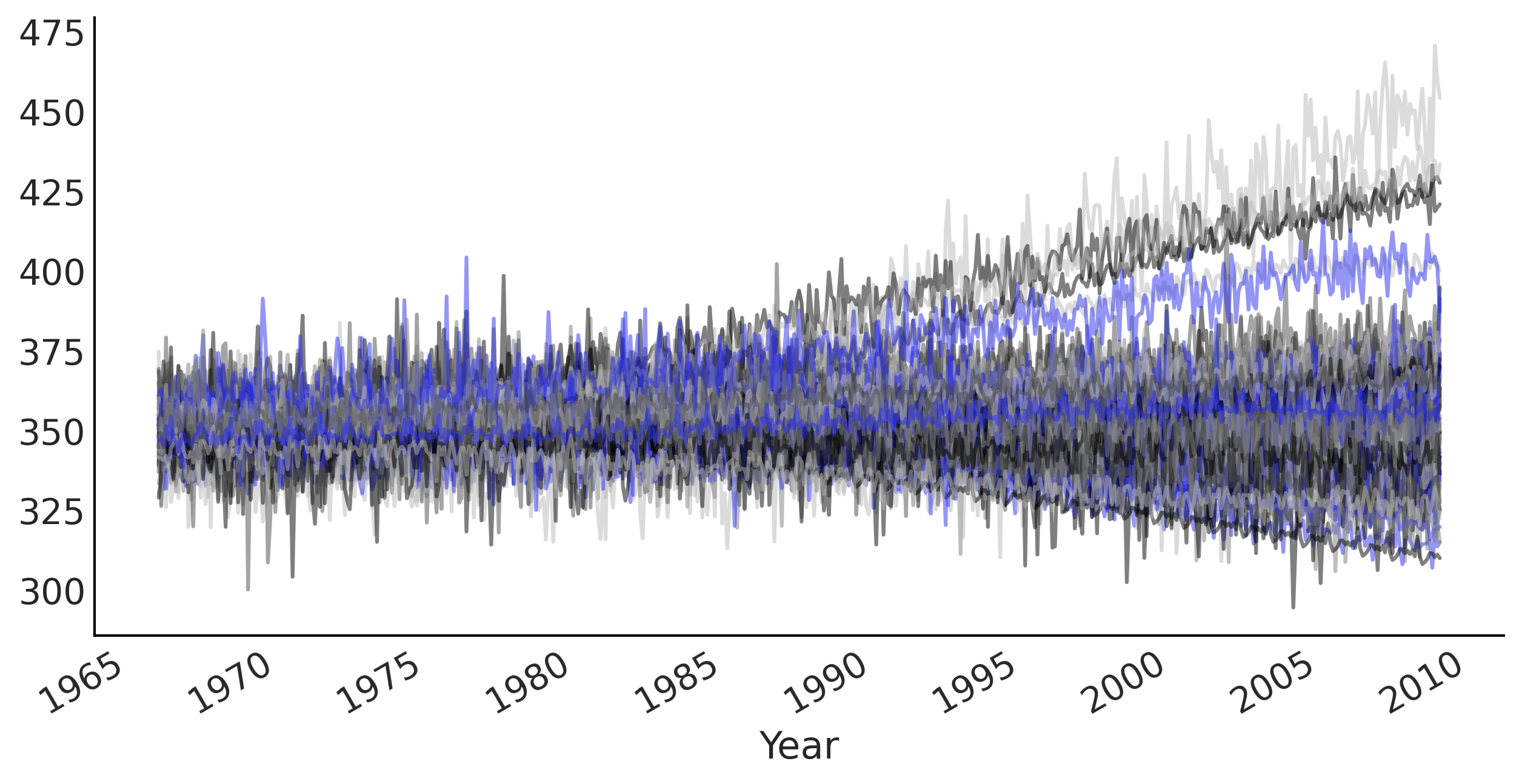
co2_by_month = pd.read_csv("../data/monthly_mauna_loa_co2.csv")
co2_by_month["date_month"] = pd.to_datetime(co2_by_month["date_month"])
co2_by_month["CO2"] = co2_by_month["CO2"].astype(np.float32)
co2_by_month.set_index("date_month", drop=True, inplace=True)

num_forecast_steps = 12 * 10  # Forecast the final ten years, given previous data
co2_by_month_training_data = co2_by_month[:-num_forecast_steps]
co2_by_month_testing_data = co2_by_month[-num_forecast_steps:]

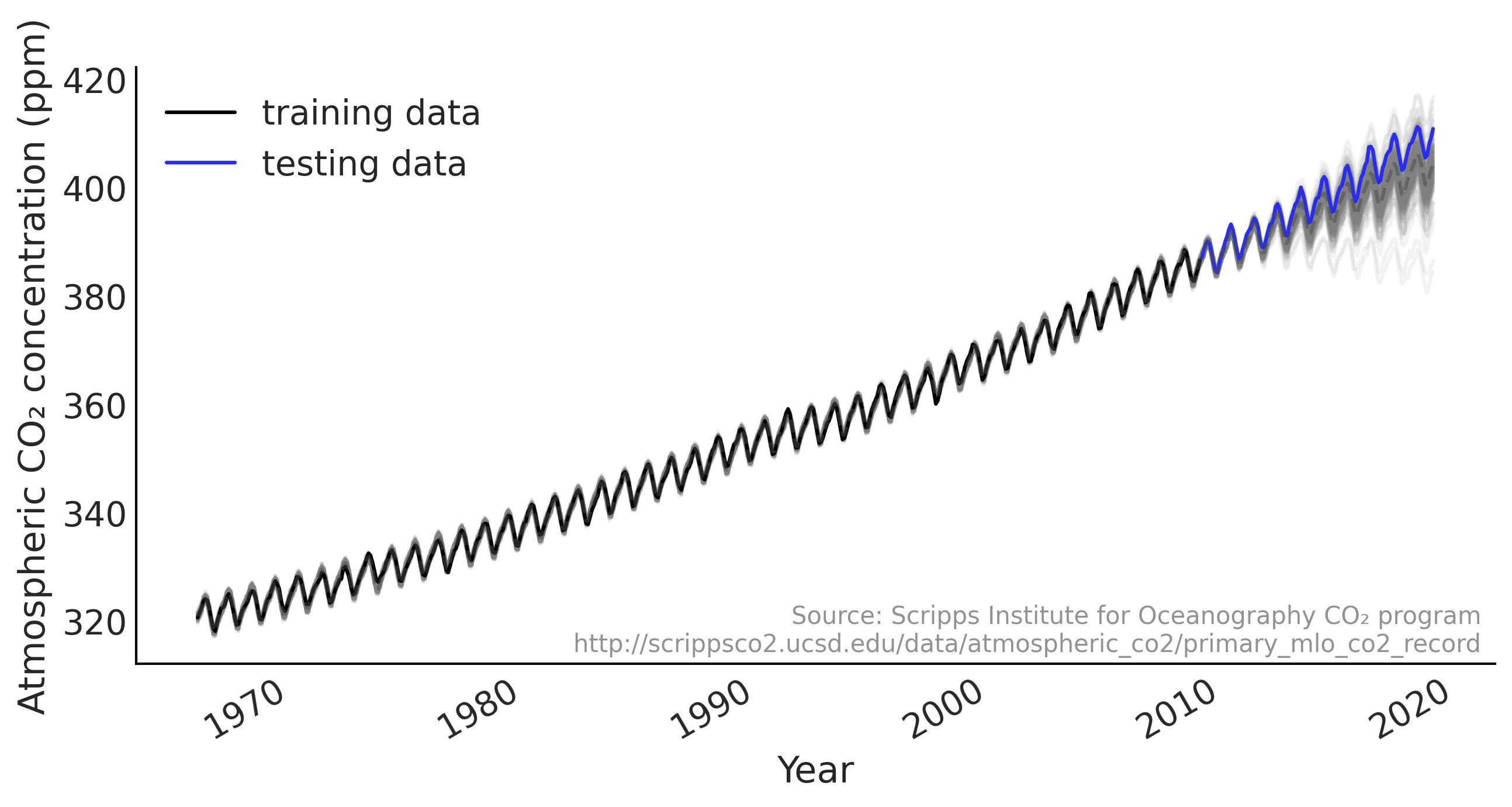
Figure 6.1

def plot_co2_data(fig_ax=None):
    if not fig_ax:
        fig, ax = plt.subplots(1, 1, figsize=(10, 5))
    else:
        fig, ax = fig_ax
    ax.plot(co2_by_month_training_data, label="training data")
    ax.plot(co2_by_month_testing_data, color="C4", label="testing data")
    ax.legend()
    ax.set(
        ylabel="Atmospheric CO₂ concentration (ppm)",
        xlabel="Year"
    )
    ax.text(0.99, .02,
            """Source: Scripps Institute for Oceanography CO₂ program
            http://scrippsco2.ucsd.edu/data/atmospheric_co2/primary_mlo_co2_record""",
            transform=ax.transAxes,
            horizontalalignment="right",
            alpha=0.5)
    fig.autofmt_xdate()
    return fig, ax


_ = plot_co2_data()
plt.savefig("img/chp06/fig1_co2_by_month.png")

/var/folders/7p/srk5qjp563l5f9mrjtp44bh800jqsw/T/ipykernel_14469/1698526664.py:19: UserWarning: This figure was using constrained_layout, but that is incompatible with subplots_adjust and/or tight_layout; disabling constrained_layout.
  fig.autofmt_xdate()

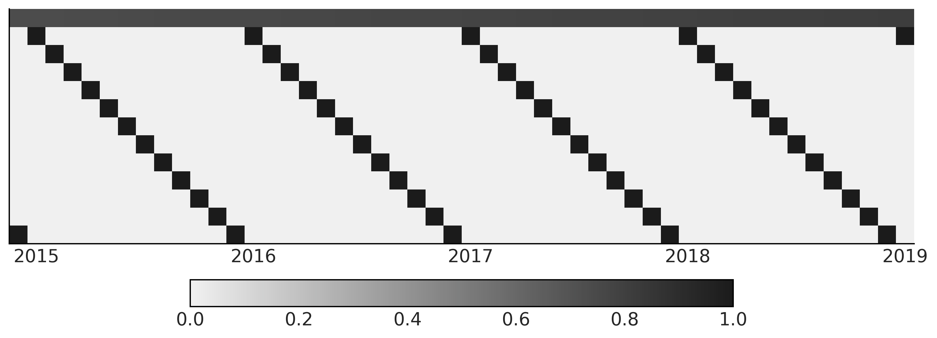
Code 6.2 and Figure 6.2

trend_all = np.linspace(0., 1., len(co2_by_month))[..., None]
trend_all = trend_all.astype(np.float32)
trend = trend_all[:-num_forecast_steps, :]

seasonality_all = pd.get_dummies(
   co2_by_month.index.month).values.astype(np.float32)
seasonality = seasonality_all[:-num_forecast_steps, :]

fig, ax = plt.subplots(figsize=(10, 4))
X_subset = np.concatenate([trend, seasonality], axis=-1)[-50:]
im = ax.imshow(X_subset.T, cmap="cet_gray_r")

label_loc = np.arange(1, 50, 12)
ax.set_xticks(label_loc)
ax.set_yticks([])
ax.set_xticklabels(co2_by_month.index.year[-50:][label_loc])
fig.colorbar(im, ax=ax, orientation="horizontal", shrink=.6)

plt.savefig("img/chp06/fig2_sparse_design_matrix.png")

Code 6.3

tfd = tfp.distributions
root = tfd.JointDistributionCoroutine.Root

@tfd.JointDistributionCoroutine
def ts_regression_model():
    intercept = yield root(tfd.Normal(0., 100., name='intercept'))
    trend_coeff = yield root(tfd.Normal(0., 10., name='trend_coeff'))
    seasonality_coeff = yield root(
        tfd.Sample(tfd.Normal(0., 1.),
                   sample_shape=seasonality.shape[-1],
                   name='seasonality_coeff'))
    noise = yield root(tfd.HalfCauchy(loc=0., scale=5., name='noise_sigma'))
    y_hat = (intercept[..., None] +
             tf.einsum('ij,...->...i', trend, trend_coeff) +
             tf.einsum('ij,...j->...i', seasonality, seasonality_coeff))
    observed = yield tfd.Independent(
        tfd.Normal(y_hat, noise[..., None]),
        reinterpreted_batch_ndims=1,
        name='observed')

# If we remove the decorator @tfd.JointDistributionCoroutine above:
# ts_regression_model = tfd.JointDistributionCoroutine(ts_regression_model)

# check shape
ts_regression_model.log_prob_parts(ts_regression_model.sample(4))

StructTuple(
  intercept=<tf.Tensor: shape=(4,), dtype=float32, numpy=array([-7.068921, -6.320923, -5.556099, -6.88211 ], dtype=float32)>,
  trend_coeff=<tf.Tensor: shape=(4,), dtype=float32, numpy=array([-3.8205433, -3.7595298, -3.3554578, -3.2555058], dtype=float32)>,
  seasonality_coeff=<tf.Tensor: shape=(4,), dtype=float32, numpy=array([-13.463518, -15.407171, -14.842403, -16.500769], dtype=float32)>,
  noise_sigma=<tf.Tensor: shape=(4,), dtype=float32, numpy=array([-5.227767 , -2.787994 , -2.855589 , -2.3863304], dtype=float32)>,
  observed=<tf.Tensor: shape=(4,), dtype=float32, numpy=array([-2344.5051, -1561.3213, -1644.2692, -1306.9598], dtype=float32)>
)

Code 6.4 and Figure 6.3

# Draw 100 prior and prior predictive samples
prior_samples = ts_regression_model.sample(100)  
prior_predictive_timeseries = prior_samples[-1]

fig, ax = plt.subplots(figsize=(10, 5))
ax.plot(co2_by_month.index[:-num_forecast_steps],
        tf.transpose(prior_predictive_timeseries), alpha=.5)
ax.set_xlabel("Year")
fig.autofmt_xdate()

plt.savefig("img/chp06/fig3_prior_predictive1.png")

/var/folders/7p/srk5qjp563l5f9mrjtp44bh800jqsw/T/ipykernel_14469/2060325595.py:9: UserWarning: This figure was using constrained_layout, but that is incompatible with subplots_adjust and/or tight_layout; disabling constrained_layout.
  fig.autofmt_xdate()

Code 6.5

run_mcmc = tf.function(
    tfp.experimental.mcmc.windowed_adaptive_nuts,
    autograph=False, jit_compile=True)

%%time
mcmc_samples, sampler_stats = run_mcmc(
    1000, ts_regression_model, n_chains=4, num_adaptation_steps=1000,
    observed=co2_by_month_training_data["CO2"].values[None, ...])

WARNING:tensorflow:From /opt/miniconda3/envs/bmcp/lib/python3.9/site-packages/tensorflow_probability/python/distributions/distribution.py:342: calling MultivariateNormalDiag.__init__ (from tensorflow_probability.python.distributions.mvn_diag) with scale_identity_multiplier is deprecated and will be removed after 2020-01-01.
Instructions for updating:
`scale_identity_multiplier` is deprecated; please combine it into `scale_diag` directly instead.

2021-11-19 17:31:24.773325: W tensorflow/compiler/tf2xla/kernels/random_ops.cc:102] Warning: Using tf.random.uniform with XLA compilation will ignore seeds; consider using tf.random.stateless_uniform instead if reproducible behavior is desired. sanitize_seed/seed
2021-11-19 17:31:24.921521: W tensorflow/compiler/tf2xla/kernels/assert_op.cc:38] Ignoring Assert operator mcmc_retry_init/assert_equal_1/Assert/AssertGuard/Assert

CPU times: user 24.4 s, sys: 596 ms, total: 25 s
Wall time: 25.2 s

regression_idata = az.from_dict(
    posterior={
        k:np.swapaxes(v.numpy(), 1, 0)
        for k, v in mcmc_samples._asdict().items()},
    sample_stats={
        k:np.swapaxes(sampler_stats[k], 1, 0)
        for k in ["target_log_prob", "diverging", "accept_ratio", "n_steps"]}
)

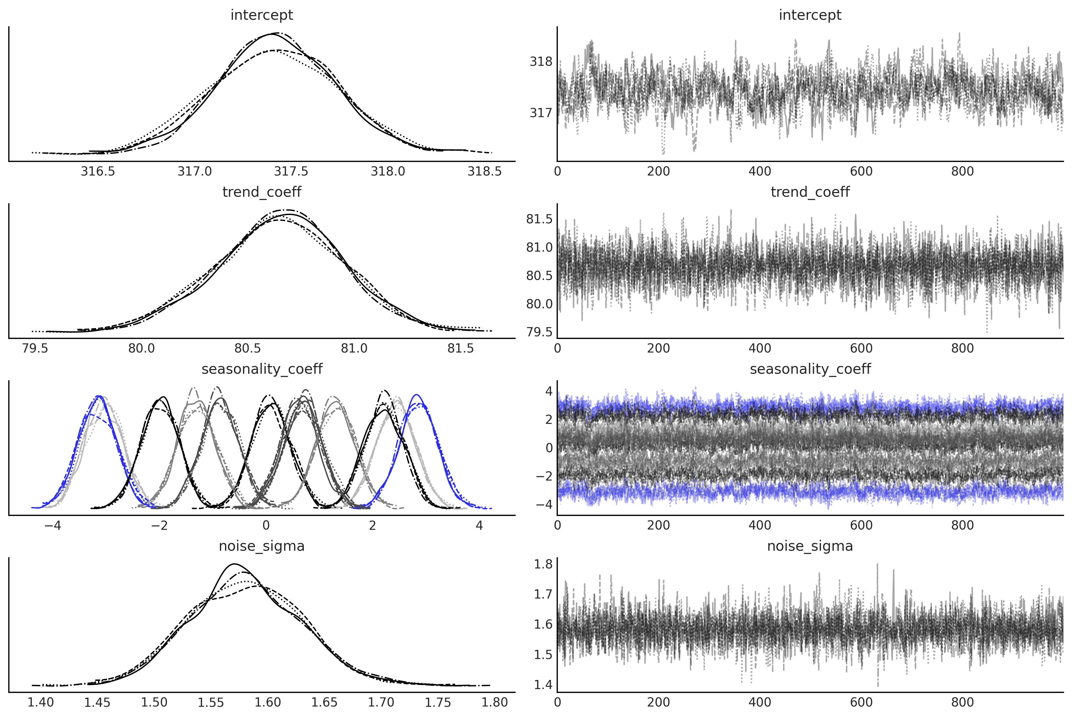
az.summary(regression_idata)

	mean	sd	hdi_3%	hdi_97%	mcse_mean	mcse_sd	ess_bulk	ess_tail	r_hat
intercept	317.417	0.323	316.828	318.046	0.014	0.010	559.0	1101.0	1.0
trend_coeff	80.648	0.299	80.096	81.225	0.005	0.003	3699.0	2994.0	1.0
seasonality_coeff[0]	0.095	0.369	-0.569	0.800	0.014	0.010	693.0	1495.0	1.0
seasonality_coeff[1]	0.647	0.366	-0.055	1.309	0.013	0.009	789.0	1580.0	1.0
seasonality_coeff[2]	1.310	0.370	0.626	2.002	0.014	0.010	712.0	1514.0	1.0
seasonality_coeff[3]	2.443	0.369	1.751	3.140	0.014	0.010	741.0	1697.0	1.0
seasonality_coeff[4]	2.861	0.366	2.168	3.549	0.014	0.010	714.0	1637.0	1.0
seasonality_coeff[5]	2.217	0.371	1.511	2.878	0.014	0.010	694.0	1493.0	1.0
seasonality_coeff[6]	0.712	0.368	0.015	1.406	0.014	0.010	710.0	1584.0	1.0
seasonality_coeff[7]	-1.296	0.365	-1.946	-0.575	0.013	0.009	749.0	1748.0	1.0
seasonality_coeff[8]	-3.041	0.365	-3.709	-2.364	0.013	0.009	783.0	1541.0	1.0
seasonality_coeff[9]	-3.157	0.365	-3.860	-2.491	0.013	0.009	793.0	1559.0	1.0
seasonality_coeff[10]	-1.987	0.362	-2.665	-1.326	0.013	0.009	729.0	1310.0	1.0
seasonality_coeff[11]	-0.858	0.364	-1.559	-0.180	0.013	0.009	747.0	1482.0	1.0
noise_sigma	1.581	0.050	1.489	1.675	0.001	0.001	4282.0	3167.0	1.0

axes = az.plot_trace(regression_idata, compact=True);

Code 6.6

# We can draw posterior predictive sample with jd.sample_distributions()
posterior_dist, posterior_and_predictive = ts_regression_model.sample_distributions(
    value=mcmc_samples)
posterior_predictive_samples = posterior_and_predictive[-1]
posterior_predictive_dist = posterior_dist[-1]

# Since we want to also plot the posterior predictive distribution for 
# each components, conditioned on both training and testing data, we
# construct the posterior predictive distribution as below:
nchains = regression_idata.posterior.dims['chain']

trend_posterior = mcmc_samples.intercept + \
    tf.einsum('ij,...->i...', trend_all, mcmc_samples.trend_coeff)
seasonality_posterior = tf.einsum(
    'ij,...j->i...', seasonality_all, mcmc_samples.seasonality_coeff)

y_hat = trend_posterior + seasonality_posterior
posterior_predictive_dist = tfd.Normal(y_hat, mcmc_samples.noise_sigma)
posterior_predictive_samples = posterior_predictive_dist.sample()

Figure 6.4

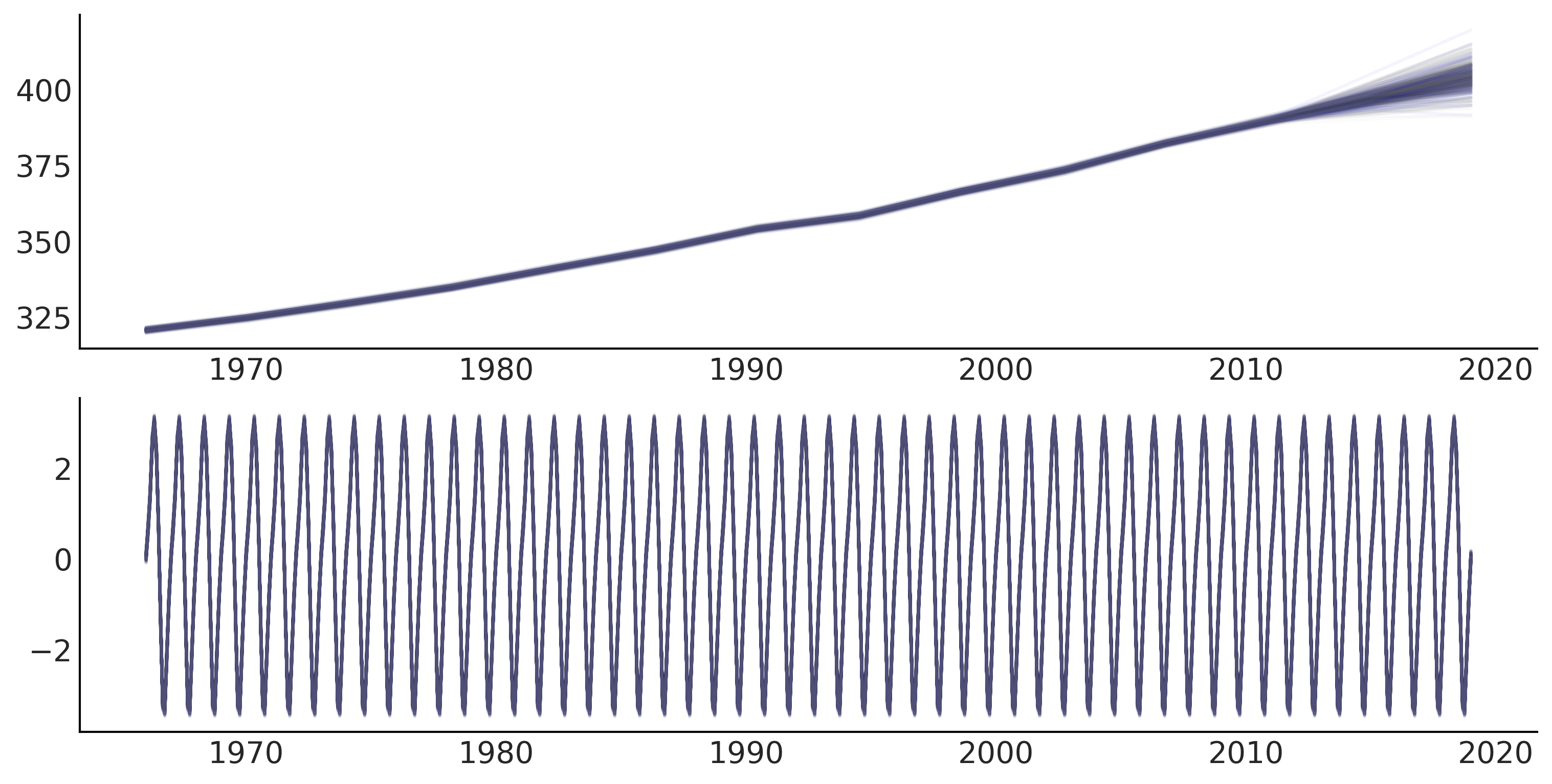
# plot components
fig, ax = plt.subplots(2, 1, figsize=(10, 5), sharex=True)

for i in range(nchains):
    ax[0].plot(co2_by_month.index[:-num_forecast_steps],
               trend_posterior[:-num_forecast_steps, -100:, i], alpha=.05)
    ax[1].plot(co2_by_month.index[:-num_forecast_steps],
               seasonality_posterior[:-num_forecast_steps, -100:, i], alpha=.05)

ax[0].set_title('Trend (Linear)')
ax[1].set_title('Seasonality (Month of the year effect)')
ax[1].set_xlabel("Year")
fig.autofmt_xdate()

plt.savefig("img/chp06/fig4_posterior_predictive_components1.png")

/var/folders/7p/srk5qjp563l5f9mrjtp44bh800jqsw/T/ipykernel_14469/865649276.py:13: UserWarning: This figure was using constrained_layout, but that is incompatible with subplots_adjust and/or tight_layout; disabling constrained_layout.
  fig.autofmt_xdate()

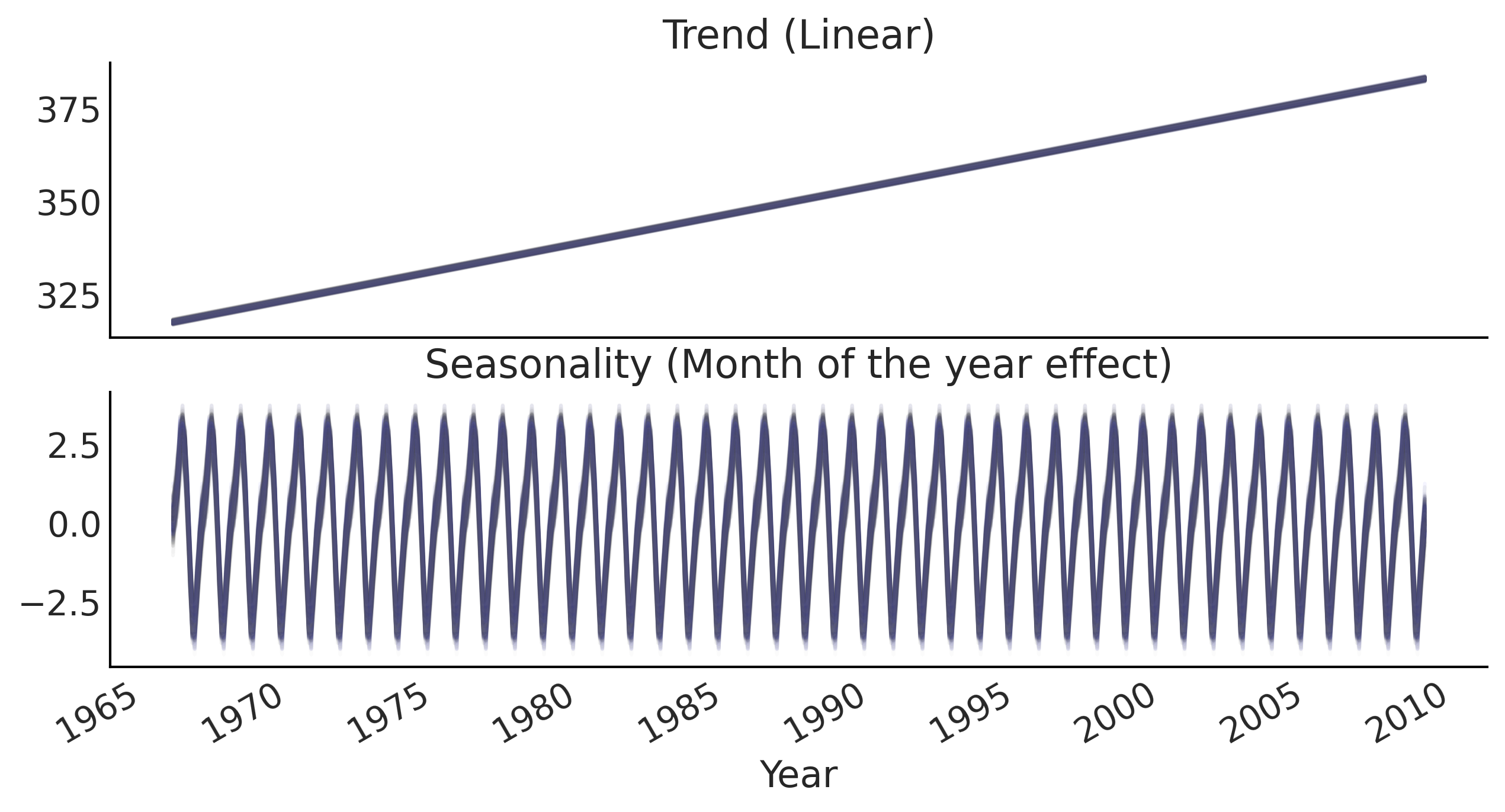
Figure 6.5

fig, ax = plt.subplots(1, 1, figsize=(10, 5))
sample_shape = posterior_predictive_samples.shape[1:]
ax.plot(co2_by_month.index,
        tf.reshape(posterior_predictive_samples,
                   [-1, tf.math.reduce_prod(sample_shape)])[:, :500],
        color='gray', alpha=.01)

plot_co2_data((fig, ax))
plt.savefig("img/chp06/fig5_posterior_predictive1.png")

/var/folders/7p/srk5qjp563l5f9mrjtp44bh800jqsw/T/ipykernel_14469/1698526664.py:19: UserWarning: This figure was using constrained_layout, but that is incompatible with subplots_adjust and/or tight_layout; disabling constrained_layout.
  fig.autofmt_xdate()

Code 6.7

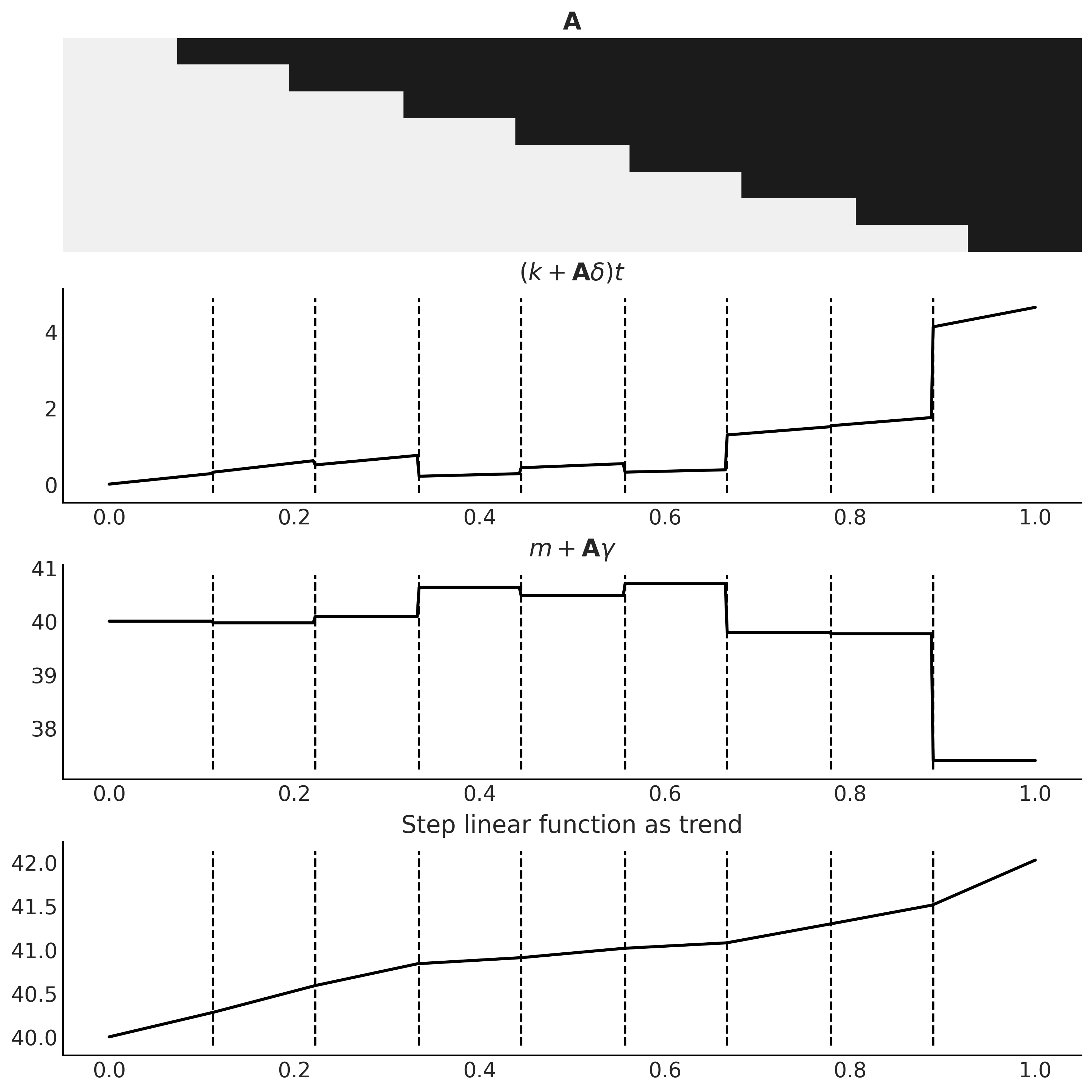
n_changepoints = 8
n_tp = 500
t = np.linspace(0, 1, n_tp)
s = np.linspace(0, 1, n_changepoints + 2)[1:-1]
A = (t[:, None] > s)

k, m = 2.5, 40
delta = np.random.laplace(.1, size=n_changepoints)
growth = (k + A @ delta) * t
offset = m + A @ (-s * delta)
trend = growth + offset

_, ax = plt.subplots(4, 1, figsize=(10, 10))
ax[0].imshow(A.T, cmap="cet_gray_r", aspect='auto', interpolation='none');
ax[0].axis('off')
ax[0].set_title(r'$\mathbf{A}$')
ax[1].plot(t, growth, lw=2)
ax[1].set_title(r'$(k + \mathbf{A}\delta) t$')
ax[2].plot(t, offset, lw=2)
ax[2].set_title(r'$m + \mathbf{A} \gamma$')
ax[3].plot(t, trend, lw=2);
ax[3].set_title('Step linear function as trend');

lines = [np.where(t > s_)[0][0] for s_ in s]
for ax_ in ax[1:]:
    ax_.vlines(t[lines], *ax_.get_ylim(), linestyles='--');
    
plt.savefig("img/chp06/fig6_step_linear_function.png");

Code 6.8 and Figure 6.7

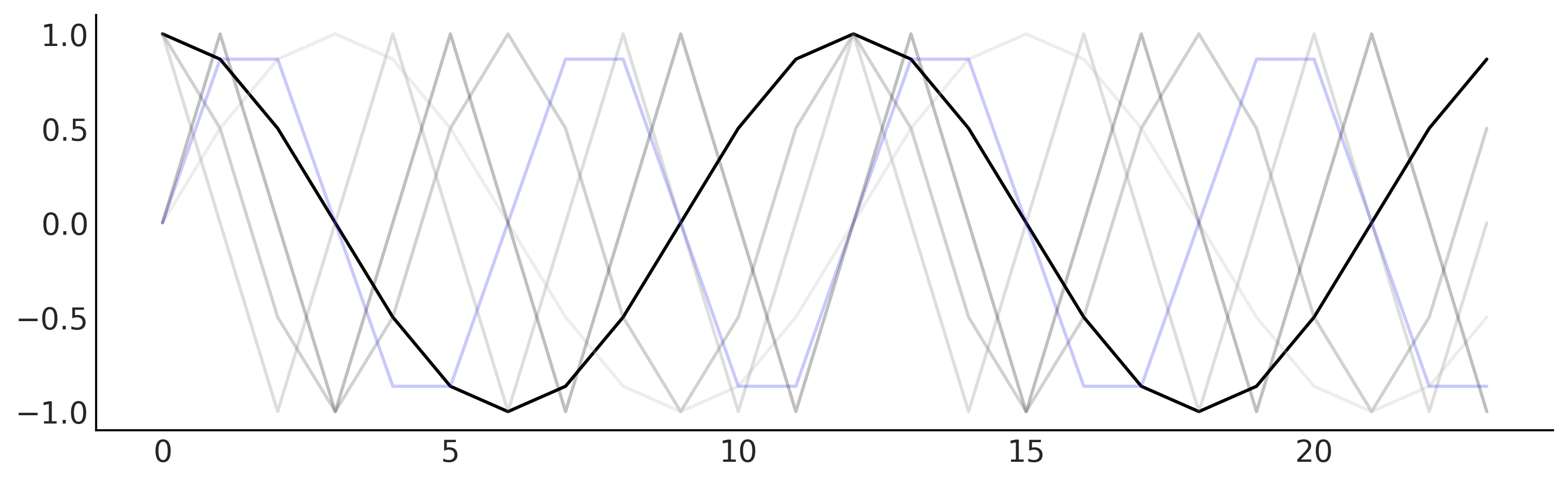
def gen_fourier_basis(t, p=365.25, n=3):
    x = 2 * np.pi * (np.arange(n) + 1) * t[:, None] / p
    return np.concatenate((np.cos(x), np.sin(x)), axis=1)

n_tp = 500
p = 12
t_monthly = np.asarray([i % p for i in range(n_tp)])
monthly_X = gen_fourier_basis(t_monthly, p=p, n=3)

fig, ax = plt.subplots(figsize=(10, 3))
ax.plot(monthly_X[:p*2, 0])
ax.plot(monthly_X[:p*2, 1:], alpha=.25)

plt.savefig("img/chp06/fig7_fourier_basis.png")

Code 6.9

# Generate trend design matrix
n_changepoints = 12

n_tp = seasonality_all.shape[0]
t = np.linspace(0, 1, n_tp, dtype=np.float32)
s = np.linspace(0, max(t), n_changepoints + 2, dtype=np.float32)[1: -1]
A = (t[:, None] > s).astype(np.float32)

# Set n=6 here so that there are 12 columns, which is the same as `seasonality_all`
X_pred = gen_fourier_basis(np.where(seasonality_all)[1],
                           p=seasonality_all.shape[-1],
                           n=6)
n_pred = X_pred.shape[-1]


def gen_gam_jd(training=True):
    @tfd.JointDistributionCoroutine
    def gam():
        beta = yield root(tfd.Sample(
            tfd.Normal(0., 1.),
            sample_shape=n_pred,
            name='beta'))
        seasonality = tf.einsum('ij,...j->...i', X_pred, beta)

        k = yield root(tfd.HalfNormal(10., name='k'))
        m = yield root(tfd.Normal(
            co2_by_month_training_data['CO2'].mean(), scale=5., name='m'))
        tau = yield root(tfd.HalfNormal(10., name='tau'))
        delta = yield tfd.Sample(tfd.Laplace(0., tau),
                                 sample_shape=n_changepoints,
                                 name='delta')

        growth_rate = k[..., None] + tf.einsum('ij,...j->...i', A, delta)
        offset = m[..., None] + tf.einsum('ij,...j->...i', A, -s * delta)
        trend = growth_rate * t + offset

        y_hat = seasonality + trend
        if training:
            y_hat = y_hat[..., :co2_by_month_training_data.shape[0]]

        noise_sigma = yield root(tfd.HalfNormal(scale=5., name='noise_sigma'))
        observed = yield tfd.Independent(
            tfd.Normal(y_hat, noise_sigma[..., None]),
            reinterpreted_batch_ndims=1,
            name='observed'
        )

    return gam


gam = gen_gam_jd()

Autoregressive Models

Figure 6.8

prior_samples = gam.sample(100)
prior_predictive_timeseries = prior_samples[-1]

fig, ax = plt.subplots(figsize=(10, 5))
ax.plot(co2_by_month.index[:-num_forecast_steps],
        tf.transpose(prior_predictive_timeseries), alpha=.5)
ax.set_xlabel("Year")
fig.autofmt_xdate()

plt.savefig("img/chp06/fig8_prior_predictive2.png");

/var/folders/7p/srk5qjp563l5f9mrjtp44bh800jqsw/T/ipykernel_14469/970221687.py:8: UserWarning: This figure was using constrained_layout, but that is incompatible with subplots_adjust and/or tight_layout; disabling constrained_layout.
  fig.autofmt_xdate()

%%time
mcmc_samples, sampler_stats = run_mcmc(
    1000, gam, n_chains=4, num_adaptation_steps=1000,
    seed=tf.constant([-12341, 62345], dtype=tf.int32),
    observed=co2_by_month_training_data.T)

2021-11-19 17:32:18.333839: W tensorflow/compiler/tf2xla/kernels/assert_op.cc:38] Ignoring Assert operator mcmc_retry_init/assert_equal_1/Assert/AssertGuard/Assert

CPU times: user 1min 4s, sys: 860 ms, total: 1min 5s
Wall time: 1min 5s

gam_idata = az.from_dict(
    posterior={
        k:np.swapaxes(v.numpy(), 1, 0)
        for k, v in mcmc_samples._asdict().items()},
    sample_stats={
        k:np.swapaxes(sampler_stats[k], 1, 0)
        for k in ["target_log_prob", "diverging", "accept_ratio", "n_steps"]}
)

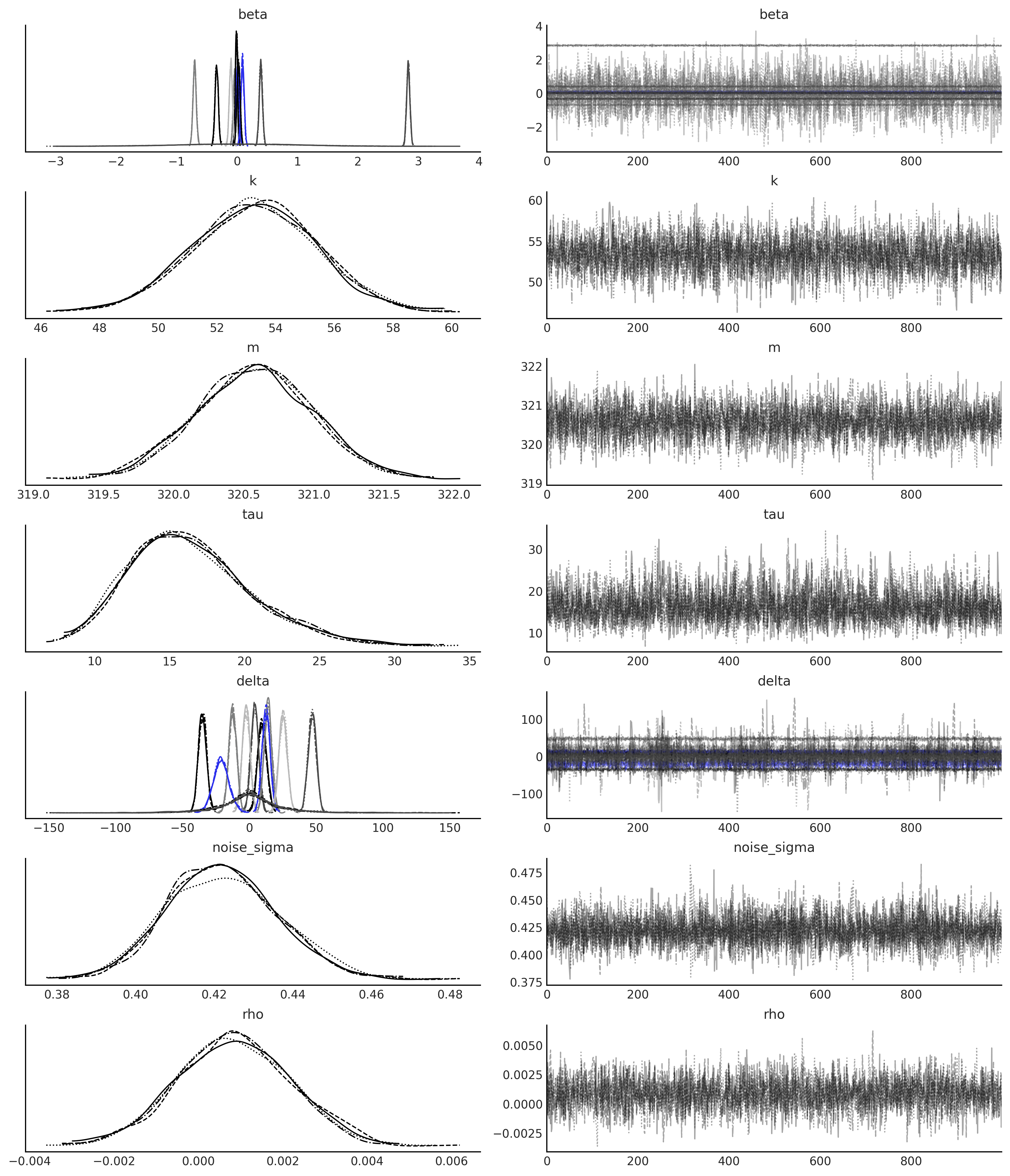
axes = az.plot_trace(gam_idata, compact=True);

gam_full = gen_gam_jd(training=False)
posterior_dists, _ = gam_full.sample_distributions(value=mcmc_samples)

# plot components
_, ax = plt.subplots(2, 1, figsize=(10, 5))

k, m, tau, delta = mcmc_samples[1:5]
growth_rate = k[..., None] + tf.einsum('ij,...j->...i', A, delta)
offset = m[..., None] + tf.einsum('ij,...j->...i', A, -s * delta)
trend_posterior = growth_rate * t + offset
seasonality_posterior = tf.einsum('ij,...j->...i', X_pred, mcmc_samples[0])

for i in range(nchains):
    ax[0].plot(co2_by_month.index,
               trend_posterior[-100:, i, :].numpy().T, alpha=.05)
    ax[1].plot(co2_by_month.index,
               seasonality_posterior[-100:, i, :].numpy().T, alpha=.05)

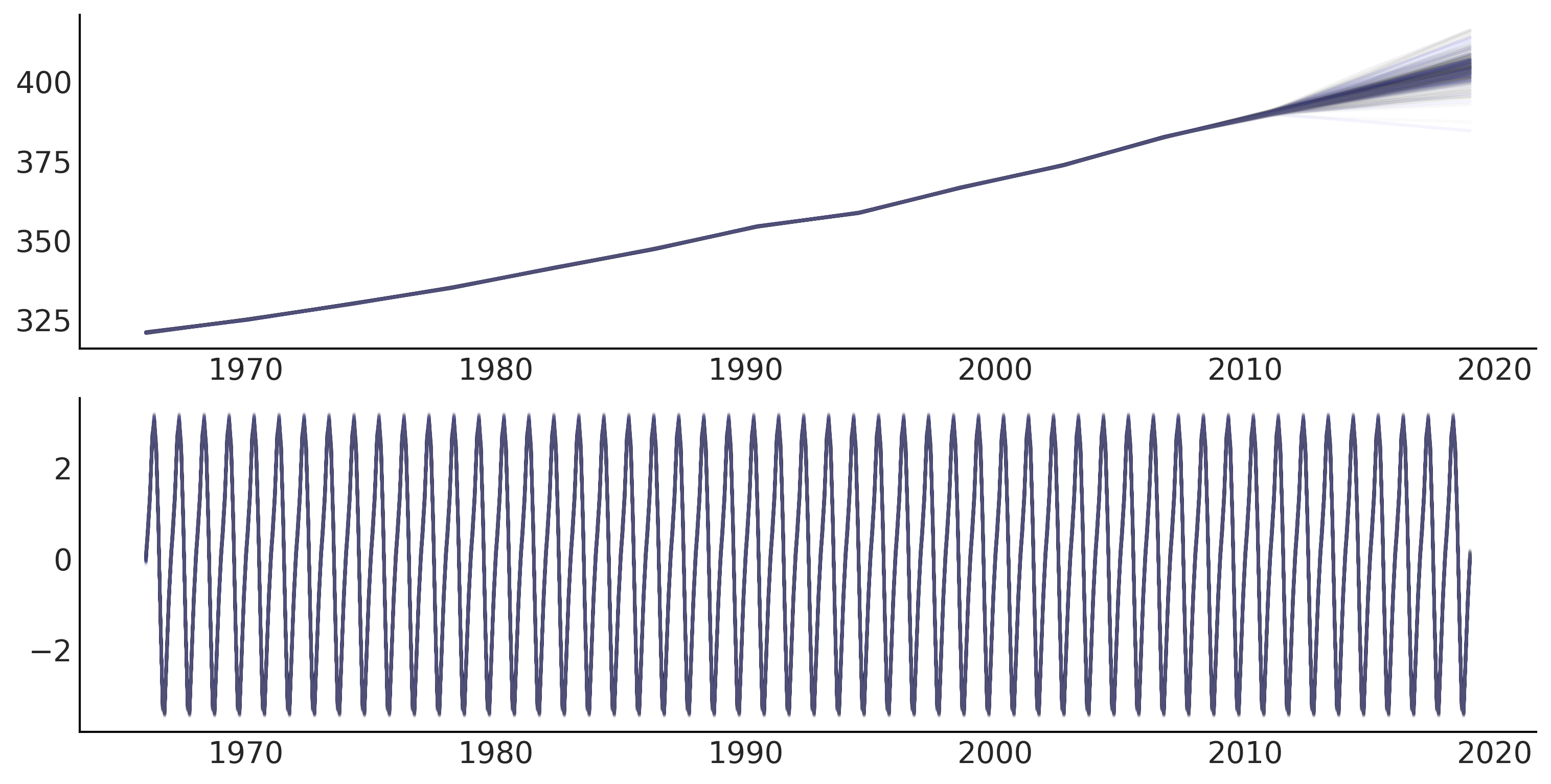
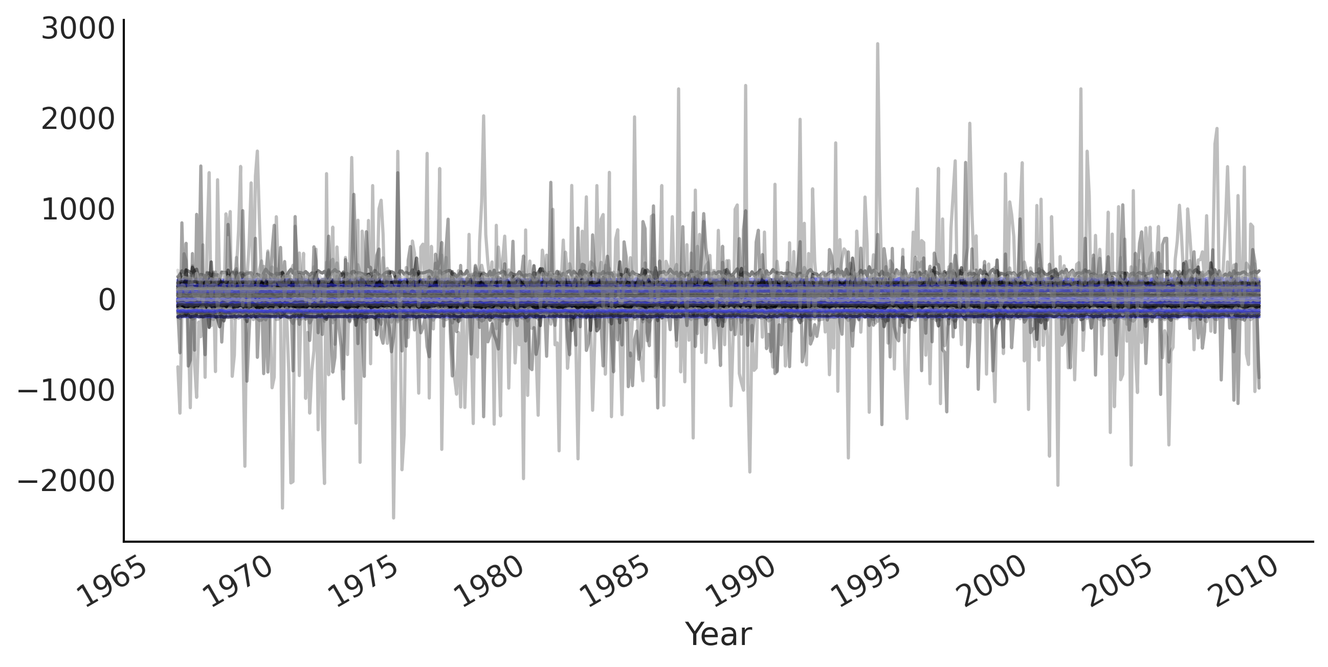
Figure 6.9

fig, ax = plt.subplots(1, 1, figsize=(10, 5))

# fitted_with_forecast = posterior_dists[-1].distribution.mean().numpy()
fitted_with_forecast = posterior_dists[-1].distribution.sample().numpy()

ax.plot(co2_by_month.index, fitted_with_forecast[-100:, 0, :].T, color='gray', alpha=.1);
ax.plot(co2_by_month.index, fitted_with_forecast[-100:, 1, :].T, color='gray', alpha=.1);

plot_co2_data((fig, ax));

average_forecast = np.mean(fitted_with_forecast, axis=(0, 1)).T
ax.plot(co2_by_month.index, average_forecast, ls='--', label='GAM forecast', alpha=.5);

plt.savefig("img/chp06/fig9_posterior_predictive2.png");

/var/folders/7p/srk5qjp563l5f9mrjtp44bh800jqsw/T/ipykernel_14469/1698526664.py:19: UserWarning: This figure was using constrained_layout, but that is incompatible with subplots_adjust and/or tight_layout; disabling constrained_layout.
  fig.autofmt_xdate()

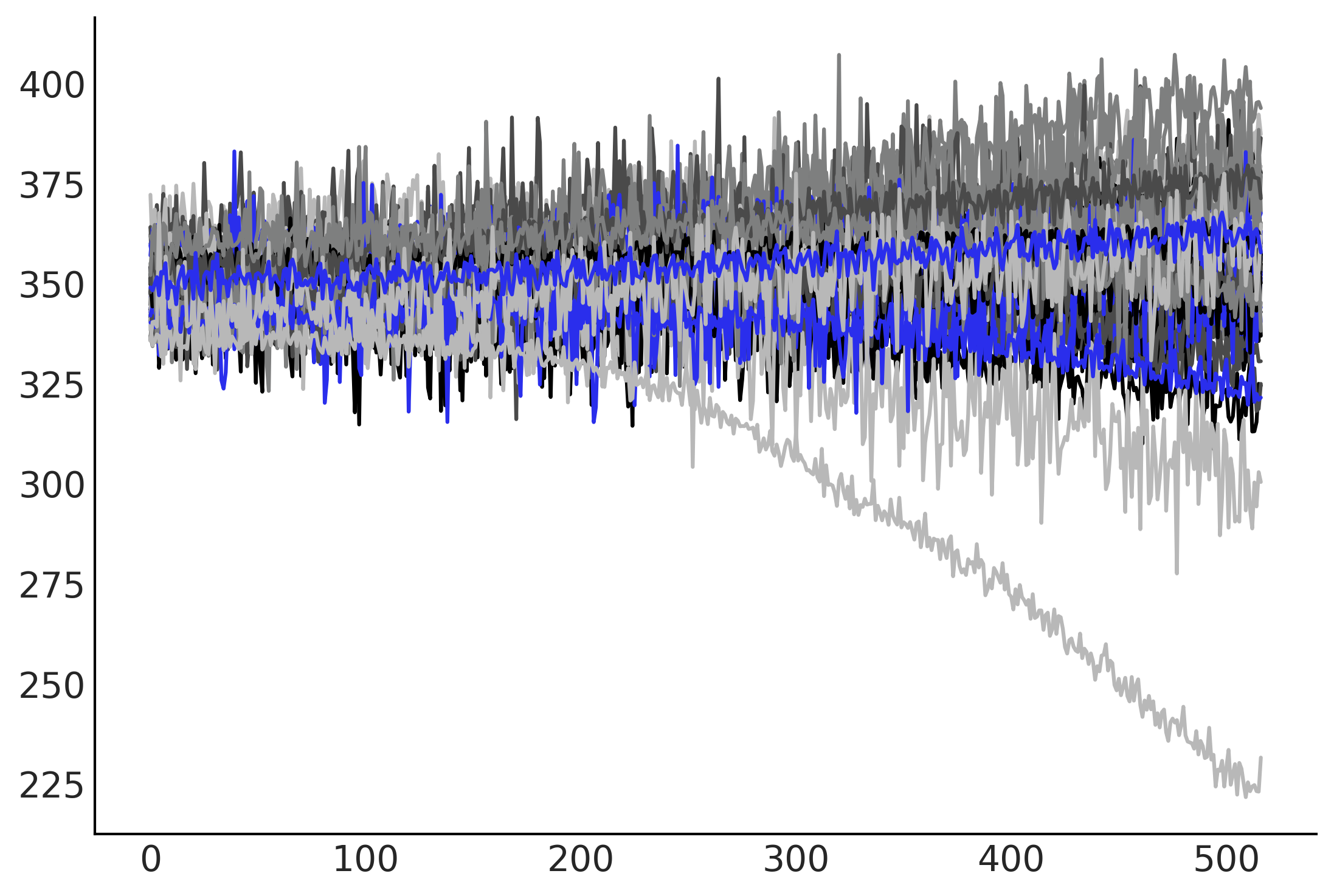
Code 6.10 and Figure 6.10

n_t = 200

@tfd.JointDistributionCoroutine
def ar1_with_forloop():
    sigma = yield root(tfd.HalfNormal(1.))
    rho = yield root(tfd.Uniform(-1., 1.))
    x0 = yield tfd.Normal(0., sigma)
    x = [x0]
    for i in range(1, n_t):
        x_i = yield tfd.Normal(x[i-1] * rho, sigma)
        x.append(x_i)

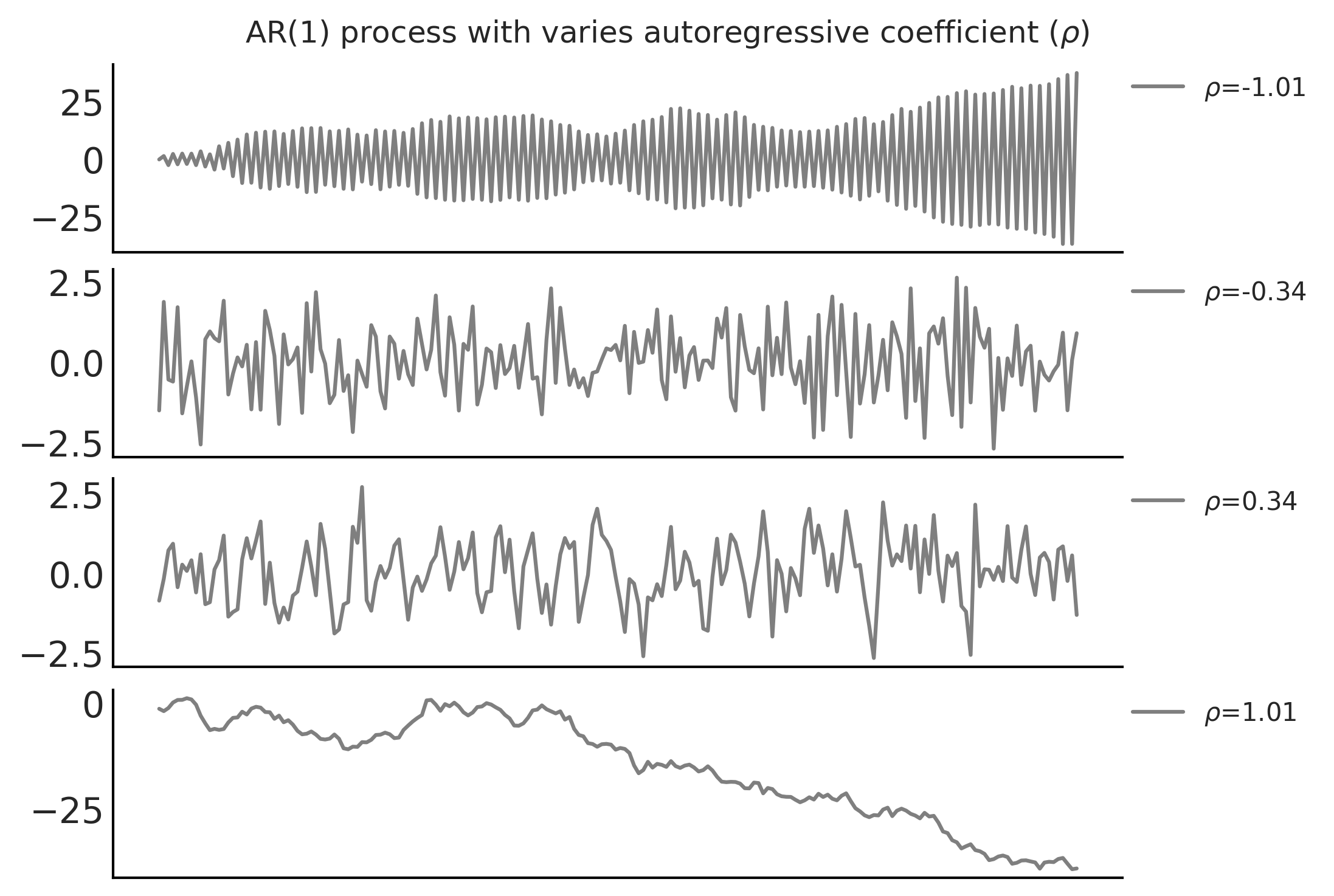
nplot = 4
fig, axes = plt.subplots(nplot, 1)
for ax, rho in zip(axes, np.linspace(-1.01, 1.01, nplot)):
    test_samples = ar1_with_forloop.sample(value=(1., rho))
    ar1_samples = tf.stack(test_samples[2:])
    ax.plot(ar1_samples, alpha=.5, label=r'$\rho$=%.2f' % rho)
    ax.legend(bbox_to_anchor=(1, 1), loc='upper left',
              borderaxespad=0., fontsize=10)
    ax.get_xaxis().set_visible(False)
fig.suptitle(r'AR(1) process with varies autoregressive coefficient ($\rho$)')

plt.savefig("img/chp06/fig10_ar1_process.png")

Code 6.11

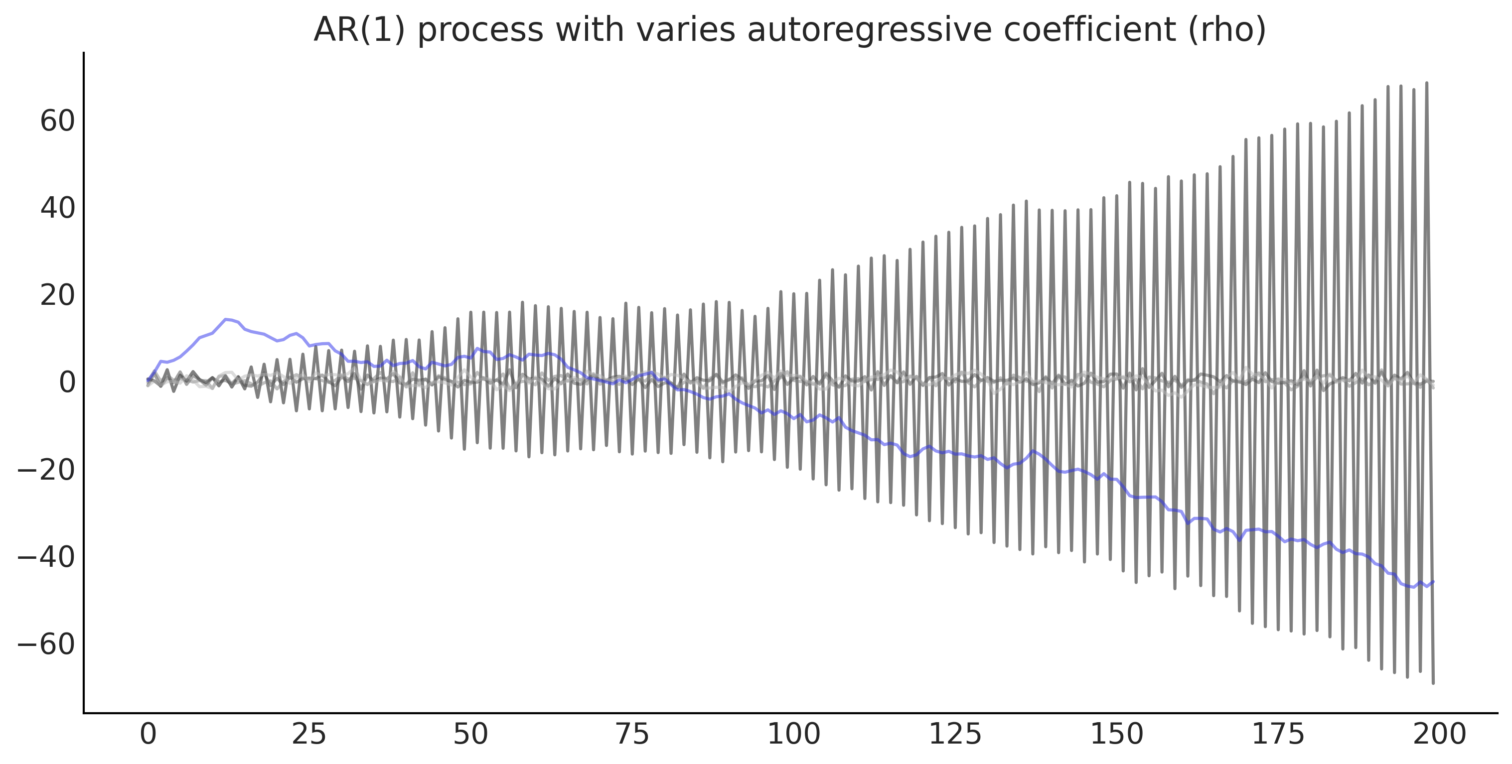
@tfd.JointDistributionCoroutine
def ar1_without_forloop():
    sigma = yield root(tfd.HalfNormal(1.))
    rho = yield root(tfd.Uniform(-1., 1.))

    def ar1_fun(x):
        # We apply the backshift operation here
        x_tm1 = tf.concat([tf.zeros_like(x[..., :1]), x[..., :-1]], axis=-1)
        loc = x_tm1 * rho[..., None]
        return tfd.Independent(tfd.Normal(loc=loc, scale=sigma[..., None]),
                               reinterpreted_batch_ndims=1)

    dist = yield tfd.Autoregressive(
        distribution_fn=ar1_fun,
        sample0=tf.zeros([n_t], dtype=rho.dtype),
        num_steps=n_t)

seed = [1000, 5234]
_, ax = plt.subplots(figsize=(10, 5))
rho = np.linspace(-1.01, 1.01, 5)
sigma = np.ones(5)
test_samples = ar1_without_forloop.sample(value=(sigma, rho), seed=seed)
ar1_samples = tf.transpose(test_samples[-1])
ax.plot(ar1_samples, alpha=.5)
ax.set_title('AR(1) process with varies autoregressive coefficient (rho)');

A more general way to implement this is to use a Lag operator \(B\)

B = np.diag(np.ones(5 - 1), -1)
B @ B

array([[0., 0., 0., 0., 0.],
       [0., 0., 0., 0., 0.],
       [1., 0., 0., 0., 0.],
       [0., 1., 0., 0., 0.],
       [0., 0., 1., 0., 0.]])

B = np.diag(np.ones(n_t - 1), -1)

@tfd.JointDistributionCoroutine
def ar1_lag_operator():
    sigma = yield root(tfd.HalfNormal(1., name='sigma'))
    rho = yield root(tfd.Uniform(-1., 1., name='rho'))

    def ar1_fun(x):
        loc = tf.einsum('ij,...j->...i', B, x) * rho[..., None]
        return tfd.Independent(tfd.Normal(loc=loc, scale=sigma[..., None]),
                               reinterpreted_batch_ndims=1)

    dist = yield tfd.Autoregressive(
            distribution_fn=ar1_fun, 
            sample0=tf.zeros([n_t], dtype=rho.dtype),
            num_steps=n_t,
            name="ar1")


_, ax = plt.subplots(figsize=(10, 5))
rho = np.linspace(-1.01, 1.01, 5)
sigma = np.ones(5)
test_samples = ar1_lag_operator.sample(value=(sigma, rho), seed=seed)
ar1_samples = tf.transpose(test_samples[-1])
ax.plot(ar1_samples, alpha=.5)
ax.set_title('AR(1) process with varies autoregressive coefficient (rho)');

Note that since we are using a stateless RNG seeding, we got the same result (yay!)

Code 6.12

def gam_trend_seasonality():
    beta = yield root(tfd.Sample(
        tfd.Normal(0., 1.),
        sample_shape=n_pred,
        name='beta'))
    seasonality = tf.einsum('ij,...j->...i', X_pred, beta)

    k = yield root(tfd.HalfNormal(10., name='k'))
    m = yield root(tfd.Normal(
        co2_by_month_training_data['CO2'].mean(), scale=5., name='m'))
    tau = yield root(tfd.HalfNormal(10., name='tau'))
    delta = yield tfd.Sample(tfd.Laplace(0., tau),
                             sample_shape=n_changepoints,
                             name='delta')

    growth_rate = k[..., None] + tf.einsum('ij,...j->...i', A, delta)
    offset = m[..., None] + tf.einsum('ij,...j->...i', A, -s * delta)
    trend = growth_rate * t + offset
    noise_sigma = yield root(tfd.HalfNormal(scale=5., name='noise_sigma'))
    return seasonality, trend, noise_sigma


def generate_gam(training=True):

    @tfd.JointDistributionCoroutine
    def gam():
        seasonality, trend, noise_sigma = yield from gam_trend_seasonality()
        y_hat = seasonality + trend
        if training:
            y_hat = y_hat[..., :co2_by_month_training_data.shape[0]]

        # likelihood
        observed = yield tfd.Independent(
            tfd.Normal(y_hat, noise_sigma[..., None]),
            reinterpreted_batch_ndims=1,
            name='observed'
        )

    return gam

gam = generate_gam()

def generate_gam_ar_likelihood(training=True):

    @tfd.JointDistributionCoroutine
    def gam_with_ar_likelihood():
        seasonality, trend, noise_sigma = yield from gam_trend_seasonality()
        y_hat = seasonality + trend
        if training:
            y_hat = y_hat[..., :co2_by_month_training_data.shape[0]]

        # Likelihood
        rho = yield root(tfd.Uniform(-1., 1., name='rho'))

        def ar_fun(y):
            loc = tf.concat([tf.zeros_like(y[..., :1]), y[..., :-1]],
                            axis=-1) * rho[..., None] + y_hat
            return tfd.Independent(
                tfd.Normal(loc=loc, scale=noise_sigma[..., None]),
                reinterpreted_batch_ndims=1)

        observed = yield tfd.Autoregressive(
            distribution_fn=ar_fun,
            sample0=tf.zeros_like(y_hat),
            num_steps=1,
            name='observed'
        )

    return gam_with_ar_likelihood


gam_with_ar_likelihood = generate_gam_ar_likelihood()

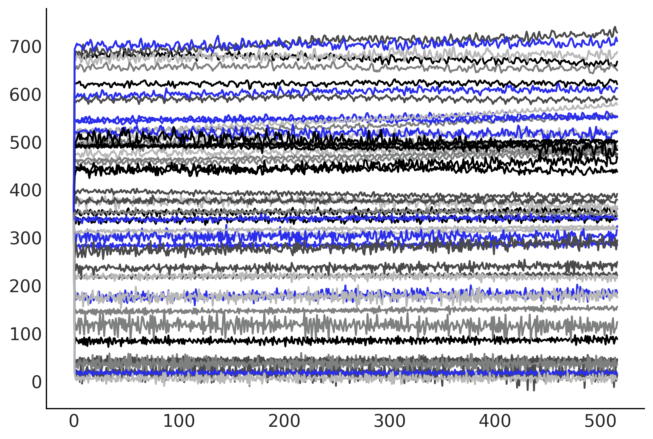
plt.plot(tf.transpose(gam_with_ar_likelihood.sample(50)[-1]));

%%time
mcmc_samples, sampler_stats = run_mcmc(
    1000, gam_with_ar_likelihood, n_chains=4, num_adaptation_steps=1000,
    seed=tf.constant([-234272345, 73564234], dtype=tf.int32),
    observed=co2_by_month_training_data.T)

2021-11-19 17:34:00.601657: W tensorflow/compiler/tf2xla/kernels/assert_op.cc:38] Ignoring Assert operator mcmc_retry_init/assert_equal_1/Assert/AssertGuard/Assert

CPU times: user 1min 19s, sys: 916 ms, total: 1min 20s
Wall time: 1min 21s

Code 6.13

gam_ar_likelihood_idata = az.from_dict(
    posterior={
        k:np.swapaxes(v.numpy(), 1, 0)
        for k, v in mcmc_samples._asdict().items()},
    sample_stats={
        k:np.swapaxes(sampler_stats[k], 1, 0)
        for k in ["target_log_prob", "diverging", "accept_ratio", "n_steps"]}
)

axes = az.plot_trace(gam_ar_likelihood_idata, compact=True);

# plot components
_, ax = plt.subplots(2, 1, figsize=(10, 5))

k, m, tau, delta = mcmc_samples[1:5]
growth_rate = k[..., None] + tf.einsum('ij,...j->...i', A, delta)
offset = m[..., None] + tf.einsum('ij,...j->...i', A, -s * delta)
trend_posterior = growth_rate * t + offset
seasonality_posterior = tf.einsum('ij,...j->...i', X_pred, mcmc_samples[0])

for i in range(nchains):
    ax[0].plot(co2_by_month.index,
               trend_posterior[-100:, i, :].numpy().T, alpha=.05)
    ax[1].plot(co2_by_month.index,
               seasonality_posterior[-100:, i, :].numpy().T, alpha=.05)

gam_with_ar_likelihood_full = generate_gam_ar_likelihood(training=False)
_, values = gam_with_ar_likelihood_full.sample_distributions(value=mcmc_samples)
fitted_with_forecast = values[-1].numpy()

fig, ax = plt.subplots(1, 1, figsize=(10, 5))

ax.plot(co2_by_month.index, fitted_with_forecast[-100:, 0, :].T, color='gray', alpha=.1);
ax.plot(co2_by_month.index, fitted_with_forecast[-100:, 1, :].T, color='gray', alpha=.1);

plot_co2_data((fig, ax));

average_forecast = np.mean(fitted_with_forecast, axis=(0, 1)).T
ax.plot(co2_by_month.index, average_forecast, ls='--', label='GAM forecast', alpha=.5);

/var/folders/7p/srk5qjp563l5f9mrjtp44bh800jqsw/T/ipykernel_14469/1698526664.py:19: UserWarning: This figure was using constrained_layout, but that is incompatible with subplots_adjust and/or tight_layout; disabling constrained_layout.
  fig.autofmt_xdate()

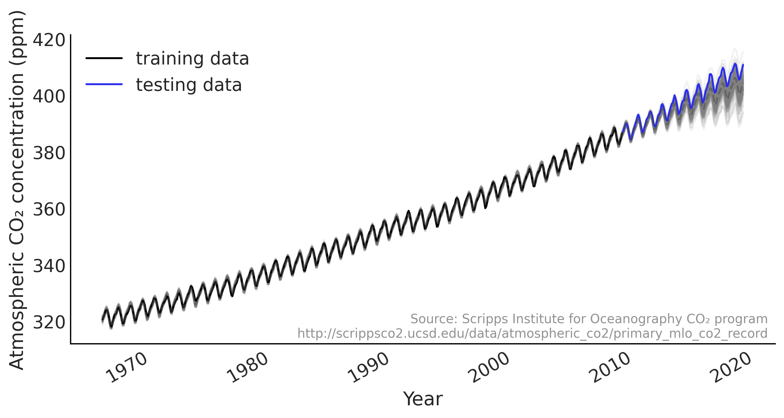
Figure 6.11

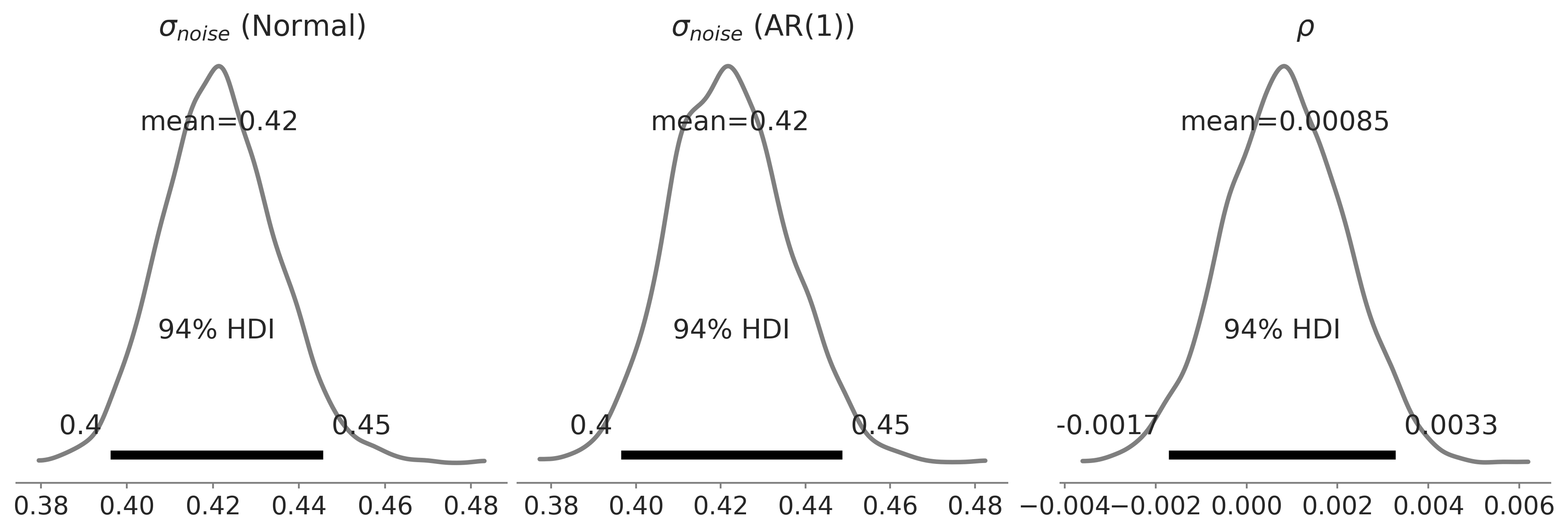
fig, axes = plt.subplots(1, 3, figsize=(4*3, 4))
az.plot_posterior(gam_idata, var_names=['noise_sigma'], alpha=.5, lw=2.5, ax=axes[0]);
axes[0].set_title(r'$\sigma_{noise}$ (Normal)')

az.plot_posterior(gam_ar_likelihood_idata, var_names=['noise_sigma', 'rho'], alpha=.5, lw=2.5, ax=axes[1:]);
axes[1].set_title(r'$\sigma_{noise}$ (AR(1))')
axes[2].set_title(r'$\rho$')

plt.savefig("img/chp06/fig11_ar1_likelihood_rho.png");

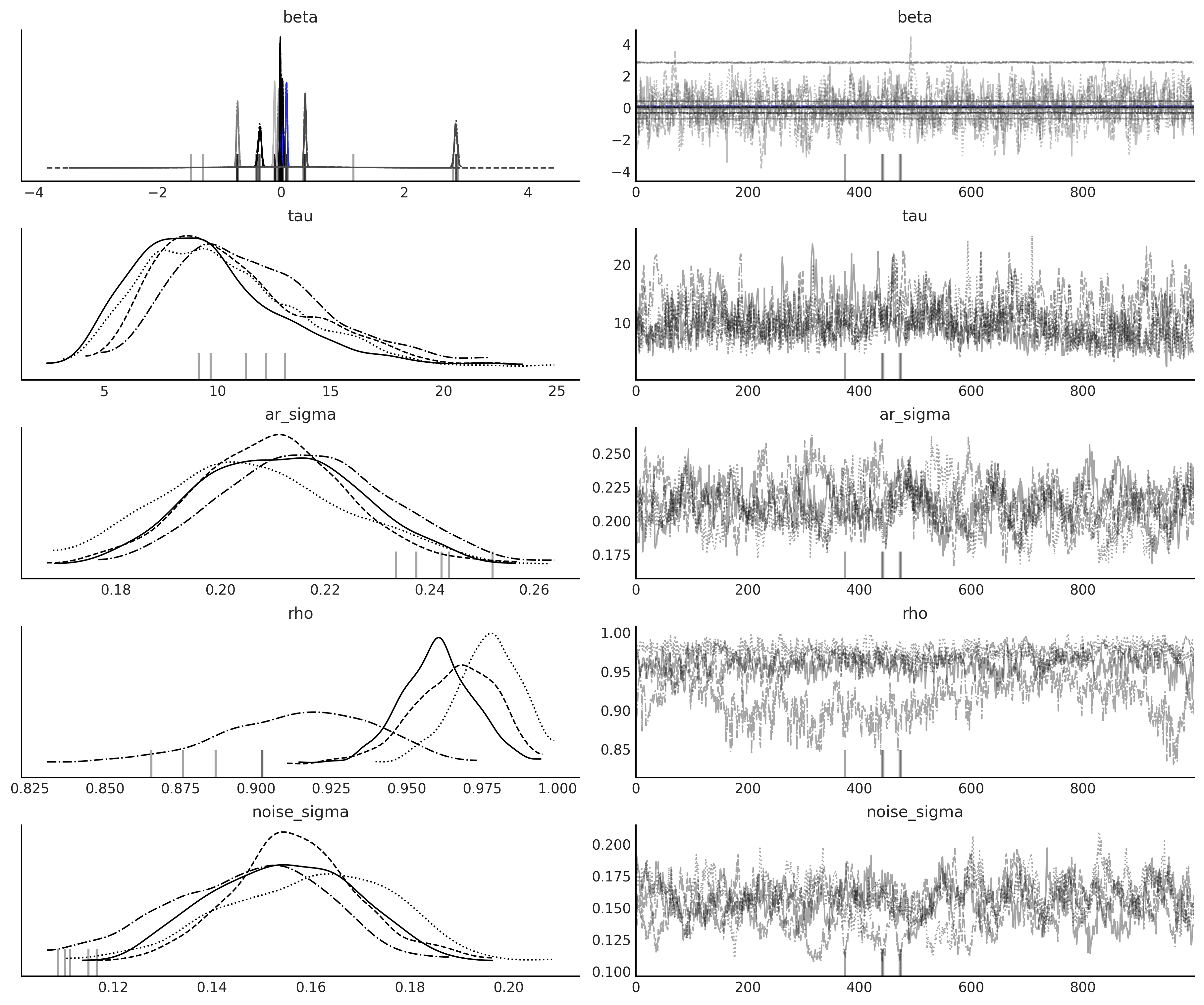
Code 6.14

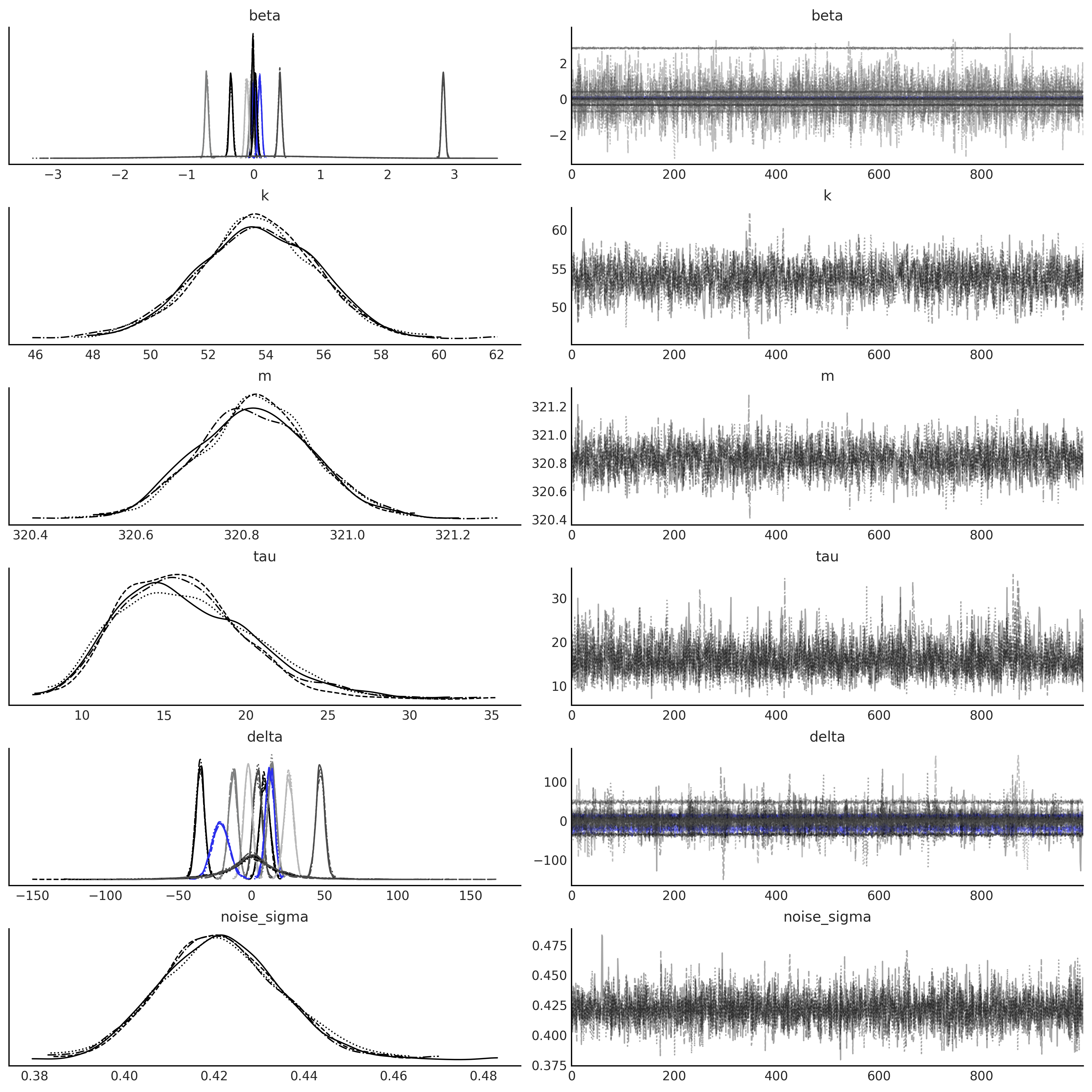
def generate_gam_ar_latent(training=True):

    @tfd.JointDistributionCoroutine
    def gam_with_latent_ar():
        seasonality, trend, noise_sigma = yield from gam_trend_seasonality()
        
        # Latent AR(1)
        ar_sigma = yield root(tfd.HalfNormal(.1, name='ar_sigma'))
        rho = yield root(tfd.Uniform(-1., 1., name='rho'))
        def ar_fun(y):
            loc = tf.concat([tf.zeros_like(y[..., :1]), y[..., :-1]],
                            axis=-1) * rho[..., None]
            return tfd.Independent(
                tfd.Normal(loc=loc, scale=ar_sigma[..., None]),
                reinterpreted_batch_ndims=1)
        temporal_error = yield tfd.Autoregressive(
            distribution_fn=ar_fun,
            sample0=tf.zeros_like(trend),
            num_steps=trend.shape[-1],
            name='temporal_error')

        # Linear prediction
        y_hat = seasonality + trend + temporal_error
        if training:
            y_hat = y_hat[..., :co2_by_month_training_data.shape[0]]

        # Likelihood
        observed = yield tfd.Independent(
            tfd.Normal(y_hat, noise_sigma[..., None]),
            reinterpreted_batch_ndims=1,
            name='observed'
        )

    return gam_with_latent_ar

gam_with_latent_ar = generate_gam_ar_latent()

plt.plot(tf.transpose(gam_with_latent_ar.sample(50)[-1]));

%%time
mcmc_samples, sampler_stats = run_mcmc(
    1000, gam_with_latent_ar, n_chains=4, num_adaptation_steps=1000,
    seed=tf.constant([36245, 734565], dtype=tf.int32),
    observed=co2_by_month_training_data.T)

2021-11-19 17:50:22.041962: W tensorflow/compiler/tf2xla/kernels/assert_op.cc:38] Ignoring Assert operator mcmc_retry_init/assert_equal_1/Assert/AssertGuard/Assert

CPU times: user 3min 9s, sys: 2.9 s, total: 3min 12s
Wall time: 3min 13s

nuts_trace_ar_latent = az.from_dict(
    posterior={
        k:np.swapaxes(v.numpy(), 1, 0)
        for k, v in mcmc_samples._asdict().items()},
    sample_stats={
        k:np.swapaxes(sampler_stats[k], 1, 0)
        for k in ["target_log_prob", "diverging", "accept_ratio", "n_steps"]}
)

axes = az.plot_trace(
    nuts_trace_ar_latent,
    var_names=['beta', 'tau', 'ar_sigma', 'rho', 'noise_sigma'],
    compact=True);

gam_with_latent_ar_full = generate_gam_ar_latent(training=False)
posterior_dists, ppc_samples = gam_with_latent_ar_full.sample_distributions(value=mcmc_samples)

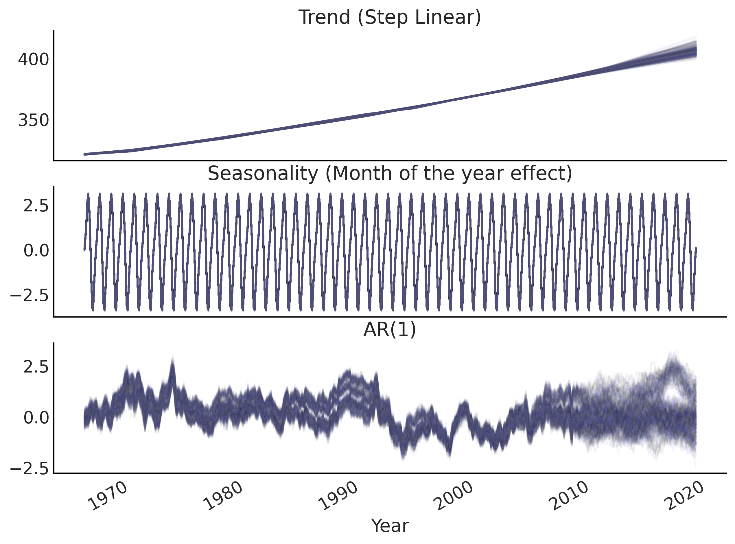
Figure 6.12

# plot components
fig, ax = plt.subplots(3, 1, figsize=(10, 7.5), sharex=True)

beta, k, m, tau, delta = mcmc_samples[:5]
growth_rate = k[..., None] + tf.einsum('ij,...j->...i', A, delta)
offset = m[..., None] + tf.einsum('ij,...j->...i', A, -s * delta)
trend_posterior = growth_rate * t + offset
seasonality_posterior = tf.einsum('ij,...j->...i', X_pred, beta)
temporal_error = mcmc_samples[-1]
# temporal_error_ = mcmc_samples[7]
# temporal_error = tf.concat([tf.zeros_like(temporal_error_[..., :1]),
#                             temporal_error_], axis=-1)

for i in range(nchains):
    ax[0].plot(co2_by_month.index, trend_posterior[-100:, i, :].numpy().T, alpha=.05);
    ax[1].plot(co2_by_month.index, seasonality_posterior[-100:, i, :].numpy().T, alpha=.05);
    ax[2].plot(co2_by_month.index, temporal_error[-100:, i, :].numpy().T, alpha=.05);

ax[0].set_title('Trend (Step Linear)')
ax[1].set_title('Seasonality (Month of the year effect)')
ax[2].set_title('AR(1)')
ax[2].set_xlabel("Year")
fig.autofmt_xdate()

plt.savefig("img/chp06/fig12_posterior_predictive_ar1.png");

/var/folders/7p/srk5qjp563l5f9mrjtp44bh800jqsw/T/ipykernel_14469/4037595605.py:23: UserWarning: This figure was using constrained_layout, but that is incompatible with subplots_adjust and/or tight_layout; disabling constrained_layout.
  fig.autofmt_xdate()

fig, ax = plt.subplots(1, 1, figsize=(10, 5))

# fitted_with_forecast = posterior_dists[-1].distribution.mean().numpy()
# fitted_with_forecast = posterior_dists[-1].distribution.sample().numpy()
fitted_with_forecast = ppc_samples[-1].numpy()

ax.plot(co2_by_month.index, fitted_with_forecast[-100:, 0, :].T, color='gray', alpha=.1);
ax.plot(co2_by_month.index, fitted_with_forecast[-100:, 1, :].T, color='gray', alpha=.1);

plot_co2_data((fig, ax));

average_forecast = np.mean(fitted_with_forecast, axis=(0, 1)).T
ax.plot(co2_by_month.index, average_forecast, ls='--', label='GAM forecast', alpha=.5);

/var/folders/7p/srk5qjp563l5f9mrjtp44bh800jqsw/T/ipykernel_14469/1698526664.py:19: UserWarning: This figure was using constrained_layout, but that is incompatible with subplots_adjust and/or tight_layout; disabling constrained_layout.
  fig.autofmt_xdate()

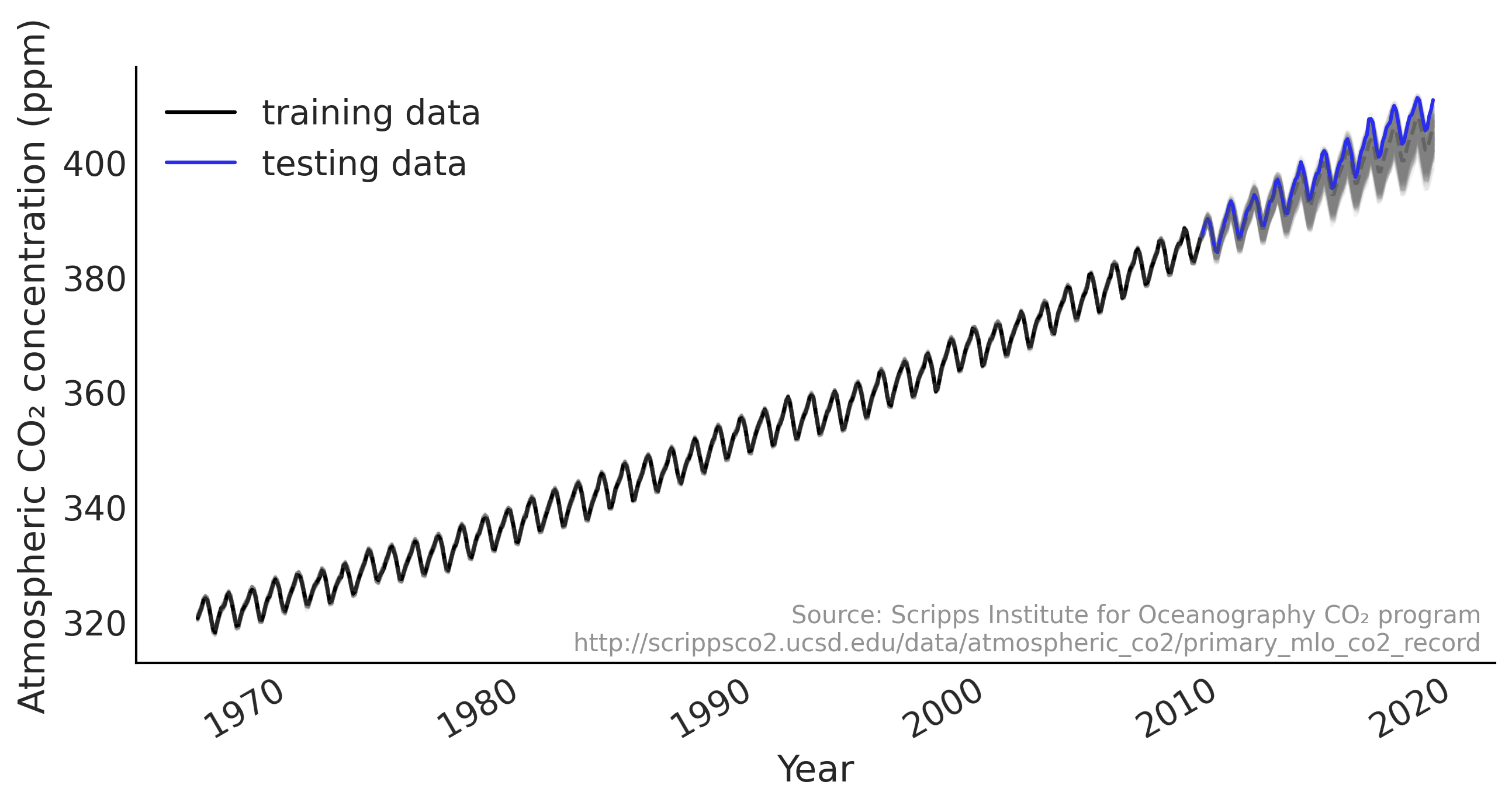
Figure 6.13

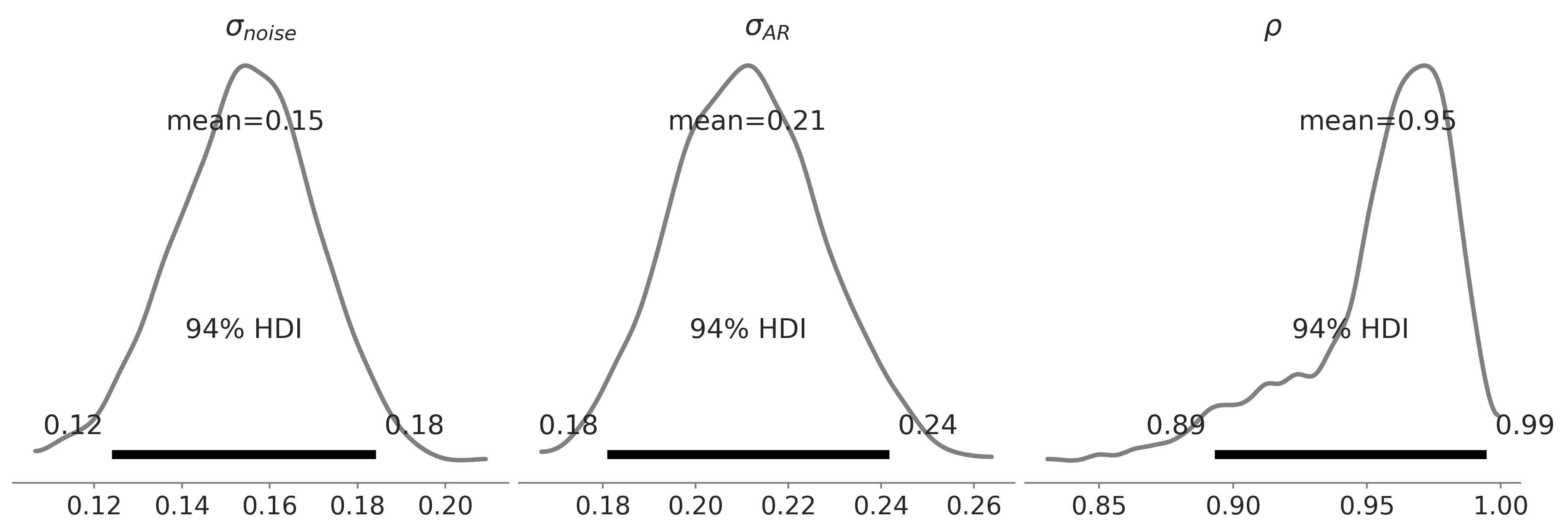
axes = az.plot_posterior(
    nuts_trace_ar_latent, 
    var_names=['noise_sigma', 'ar_sigma', 'rho'], 
    alpha=.5, lw=2.5, 
    figsize=(4*3, 4));
axes[0].set_title(r'$\sigma_{noise}$')
axes[1].set_title(r'$\sigma_{AR}$')
axes[2].set_title(r'$\rho$')

plt.savefig("img/chp06/fig13_ar1_likelihood_rho2.png");

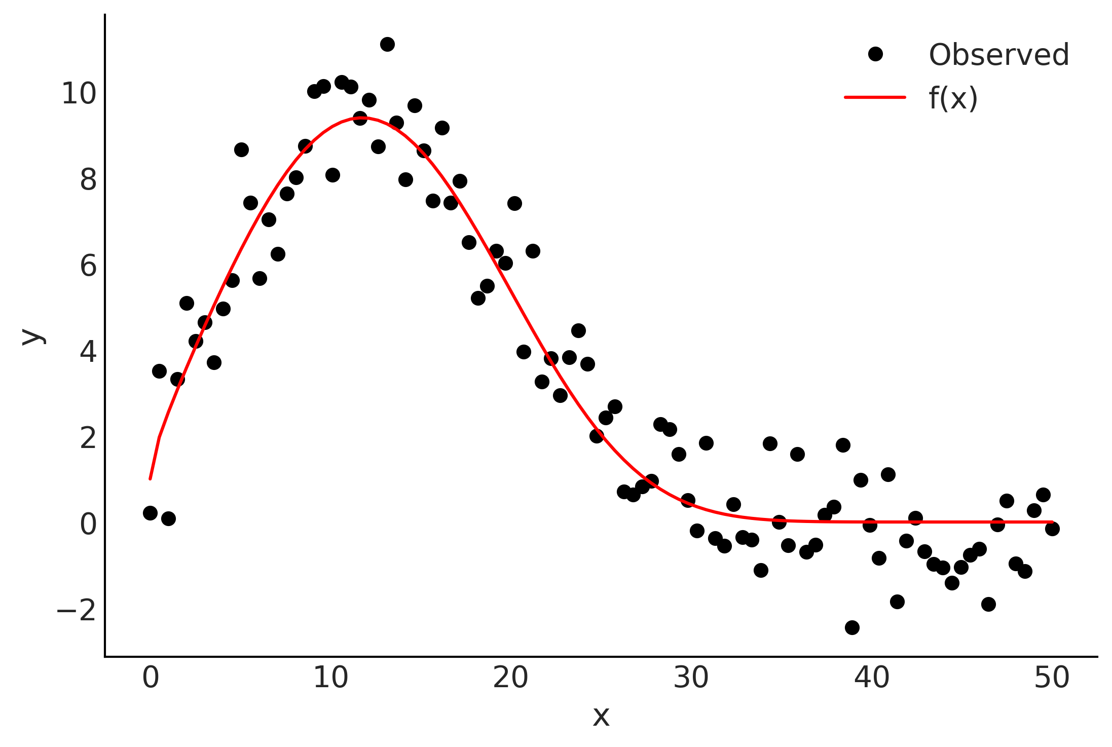
Reflection on autoregressive and smoothing

num_steps = 100

x = np.linspace(0, 50, num_steps)
f = np.exp(1.0 + np.power(x, 0.5) - np.exp(x/15.0))
y = f + np.random.normal(scale=1.0, size=x.shape)

plt.plot(x, y, 'ok', label='Observed')
plt.plot(x, f, 'r', label='f(x)')
plt.legend()
plt.xlabel('x');
plt.ylabel('y');

Code 6.15

@tfd.JointDistributionCoroutine
def smoothing_grw():
    alpha = yield root(tfd.Beta(5, 1.))
    variance = yield root(tfd.HalfNormal(10.))
    sigma0 = tf.sqrt(variance * alpha)
    sigma1 = tf.sqrt(variance * (1. - alpha))
    z = yield tfd.Sample(tfd.Normal(0., sigma0), num_steps)
    observed = yield tfd.Independent(
        tfd.Normal(tf.math.cumsum(z, axis=-1), sigma1[..., None]),
        name='observed'
    )

%%time
mcmc_samples, sampler_stats = run_mcmc(
    1000, smoothing_grw, n_chains=4, num_adaptation_steps=1000,
    observed=tf.constant(y[None, ...], dtype=tf.float32))

WARNING:tensorflow:@custom_gradient grad_fn has 'variables' in signature, but no ResourceVariables were used on the forward pass.
WARNING:tensorflow:@custom_gradient grad_fn has 'variables' in signature, but no ResourceVariables were used on the forward pass.
WARNING:tensorflow:From /opt/miniconda3/envs/bmcp/lib/python3.9/site-packages/tensorflow_probability/python/distributions/distribution.py:342: calling Independent.__init__ (from tensorflow_probability.python.distributions.independent) with reinterpreted_batch_ndims=None is deprecated and will be removed after 2022-03-01.
Instructions for updating:
Please pass an integer value for `reinterpreted_batch_ndims`. The current behavior corresponds to `reinterpreted_batch_ndims=tf.size(distribution.batch_shape_tensor()) - 1`.
WARNING:tensorflow:@custom_gradient grad_fn has 'variables' in signature, but no ResourceVariables were used on the forward pass.
WARNING:tensorflow:@custom_gradient grad_fn has 'variables' in signature, but no ResourceVariables were used on the forward pass.
WARNING:tensorflow:@custom_gradient grad_fn has 'variables' in signature, but no ResourceVariables were used on the forward pass.
WARNING:tensorflow:@custom_gradient grad_fn has 'variables' in signature, but no ResourceVariables were used on the forward pass.
WARNING:tensorflow:@custom_gradient grad_fn has 'variables' in signature, but no ResourceVariables were used on the forward pass.
WARNING:tensorflow:@custom_gradient grad_fn has 'variables' in signature, but no ResourceVariables were used on the forward pass.
WARNING:tensorflow:@custom_gradient grad_fn has 'variables' in signature, but no ResourceVariables were used on the forward pass.

2021-11-19 17:56:39.831415: W tensorflow/core/framework/op_kernel.cc:1745] OP_REQUIRES failed at functional_ops.cc:373 : INTERNAL: No function library
2021-11-19 17:56:39.831472: W tensorflow/core/framework/op_kernel.cc:1745] OP_REQUIRES failed at functional_ops.cc:373 : INTERNAL: No function library
2021-11-19 17:56:39.852216: W tensorflow/core/framework/op_kernel.cc:1745] OP_REQUIRES failed at functional_ops.cc:373 : INTERNAL: No function library
2021-11-19 17:56:39.852258: W tensorflow/core/framework/op_kernel.cc:1745] OP_REQUIRES failed at functional_ops.cc:373 : INTERNAL: No function library
2021-11-19 17:56:39.874546: W tensorflow/core/framework/op_kernel.cc:1745] OP_REQUIRES failed at functional_ops.cc:373 : INTERNAL: No function library
2021-11-19 17:56:39.874599: W tensorflow/core/framework/op_kernel.cc:1745] OP_REQUIRES failed at functional_ops.cc:373 : INTERNAL: No function library
2021-11-19 17:56:39.885913: W tensorflow/core/framework/op_kernel.cc:1745] OP_REQUIRES failed at functional_ops.cc:373 : INTERNAL: No function library
2021-11-19 17:56:39.885967: W tensorflow/core/framework/op_kernel.cc:1745] OP_REQUIRES failed at functional_ops.cc:373 : INTERNAL: No function library
2021-11-19 17:56:39.920939: W tensorflow/core/framework/op_kernel.cc:1745] OP_REQUIRES failed at functional_ops.cc:373 : INTERNAL: No function library
2021-11-19 17:56:39.920993: W tensorflow/core/framework/op_kernel.cc:1745] OP_REQUIRES failed at functional_ops.cc:373 : INTERNAL: No function library
2021-11-19 17:56:40.343209: W tensorflow/core/framework/op_kernel.cc:1745] OP_REQUIRES failed at functional_ops.cc:373 : INTERNAL: No function library
2021-11-19 17:56:40.343251: W tensorflow/core/framework/op_kernel.cc:1745] OP_REQUIRES failed at functional_ops.cc:373 : INTERNAL: No function library
2021-11-19 17:56:40.350681: W tensorflow/core/framework/op_kernel.cc:1745] OP_REQUIRES failed at functional_ops.cc:373 : INTERNAL: No function library
2021-11-19 17:56:40.350794: W tensorflow/core/framework/op_kernel.cc:1745] OP_REQUIRES failed at functional_ops.cc:373 : INTERNAL: No function library
2021-11-19 17:56:40.357544: W tensorflow/core/framework/op_kernel.cc:1745] OP_REQUIRES failed at functional_ops.cc:373 : INTERNAL: No function library
2021-11-19 17:56:40.357614: W tensorflow/core/framework/op_kernel.cc:1745] OP_REQUIRES failed at functional_ops.cc:373 : INTERNAL: No function library
2021-11-19 17:56:40.366483: W tensorflow/core/framework/op_kernel.cc:1745] OP_REQUIRES failed at functional_ops.cc:373 : INTERNAL: No function library
2021-11-19 17:56:40.366524: W tensorflow/core/framework/op_kernel.cc:1745] OP_REQUIRES failed at functional_ops.cc:373 : INTERNAL: No function library
2021-11-19 17:56:40.611639: W tensorflow/compiler/tf2xla/kernels/assert_op.cc:38] Ignoring Assert operator mcmc_retry_init/assert_equal_1/Assert/AssertGuard/Assert

WARNING:tensorflow:5 out of the last 9 calls to <function windowed_adaptive_nuts at 0x7fae934af550> triggered tf.function retracing. Tracing is expensive and the excessive number of tracings could be due to (1) creating @tf.function repeatedly in a loop, (2) passing tensors with different shapes, (3) passing Python objects instead of tensors. For (1), please define your @tf.function outside of the loop. For (2), @tf.function has experimental_relax_shapes=True option that relaxes argument shapes that can avoid unnecessary retracing. For (3), please refer to https://www.tensorflow.org/guide/function#controlling_retracing and https://www.tensorflow.org/api_docs/python/tf/function for  more details.
CPU times: user 36.1 s, sys: 342 ms, total: 36.4 s
Wall time: 36.5 s

_, ax = plt.subplots(2, 1, figsize=(10, 5))
ax[0].plot(mcmc_samples[0], alpha=.5)
ax[1].plot(mcmc_samples[1], alpha=.5);

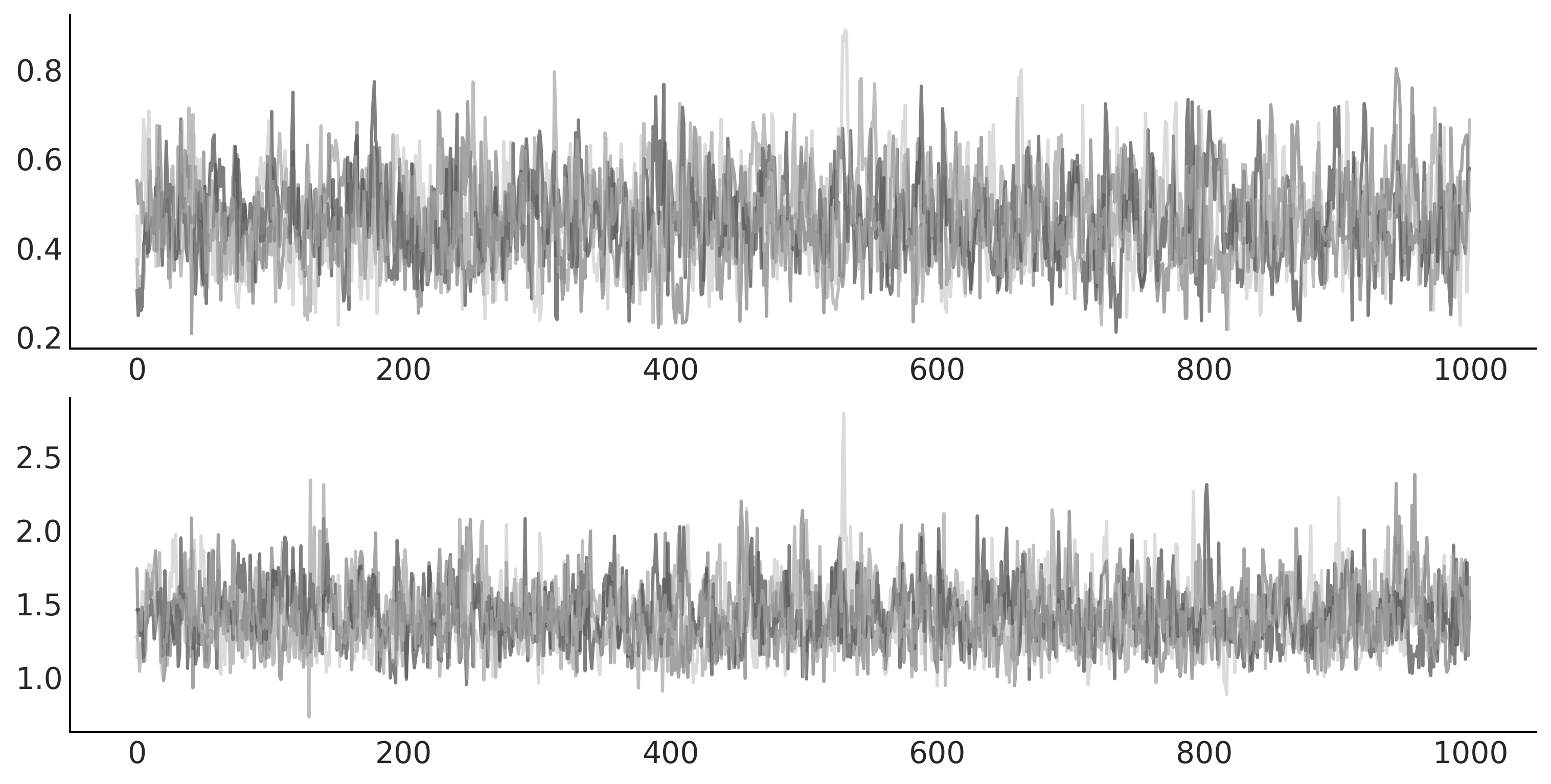
Figure 6.14

nsample, nchain = mcmc_samples[-1].shape[:2]

z = tf.reshape(tf.math.cumsum(mcmc_samples[-1], axis=-1), [nsample*nchain, -1])
lower, upper = np.percentile(z, [5, 95], axis=0)

_, ax = plt.subplots(figsize=(10, 4))

ax.plot(x, y, 'o', label='Observed')
ax.plot(x, f, label='f(x)')
ax.fill_between(x, lower, upper, color='C1', alpha=.25)
ax.plot(x, tf.reduce_mean(z, axis=0), color='C4', ls='--', label='z')
ax.legend()
ax.set_xlabel('x');
ax.set_ylabel('y');

plt.savefig("img/chp06/fig14_smoothing_with_gw.png");

SARIMA

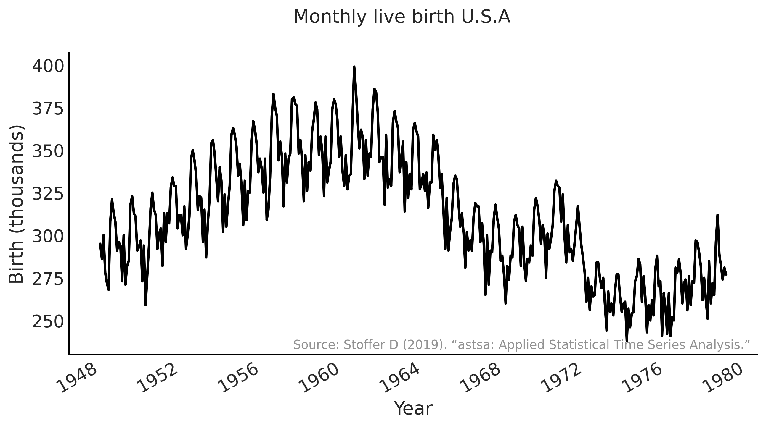
Code 6.16 and Figure 6.15

us_monthly_birth = pd.read_csv("../data/monthly_birth_usa.csv")
us_monthly_birth["date_month"] = pd.to_datetime(us_monthly_birth["date_month"])
us_monthly_birth.set_index("date_month", drop=True, inplace=True)

def plot_birth_data(fig_ax=None):
    if not fig_ax:
        fig, ax = plt.subplots(1, 1, figsize=(10, 5))
    else:
        fig, ax = fig_ax
    
    ax.plot(us_monthly_birth, lw=2)
    ax.set_ylabel("Birth (thousands)")
    ax.set_xlabel("Year")
    fig.suptitle("Monthly live birth U.S.A",
                 fontsize=15)
    ax.text(0.99, .02,
            "Source: Stoffer D (2019). “astsa: Applied Statistical Time Series Analysis.”",
            transform=ax.transAxes,
            horizontalalignment="right",
            alpha=0.5)
    fig.autofmt_xdate()
    return fig, ax


_ = plot_birth_data()

plt.savefig("img/chp06/fig15_birth_by_month.png")

/var/folders/7p/srk5qjp563l5f9mrjtp44bh800jqsw/T/ipykernel_14469/1306182099.py:21: UserWarning: This figure was using constrained_layout, but that is incompatible with subplots_adjust and/or tight_layout; disabling constrained_layout.
  fig.autofmt_xdate()

y ~ Sarima(1,1,1)(1,1,1)[12]

Code 6.17

# y ~ Sarima(1,1,1)(1,1,1)[12]
p, d, q = (1, 1, 1)
P, D, Q, period = (1, 1, 1, 12)
# Time series data: us_monthly_birth.shape = (372,)
observed = us_monthly_birth["birth_in_thousands"].values
# Integrated to seasonal order $D$
for _ in range(D):
    observed = observed[period:] - observed[:-period]
# Integrated to order $d$
observed = tf.constant(np.diff(observed, n=d), tf.float32)

r = max(p, q, P * period, Q * period)
def likelihood(mu0, sigma, phi, theta, sphi, stheta):
    batch_shape = tf.shape(mu0)
    y_extended = tf.concat(
        [tf.zeros(tf.concat([[r], batch_shape], axis=0), dtype=mu0.dtype),
        tf.einsum('...,j->j...',
                  tf.ones_like(mu0, dtype=observed.dtype),
                  observed)],
        axis=0)
    eps_t = tf.zeros_like(y_extended, dtype=observed.dtype)

    def arma_onestep(t, eps_t):
        t_shift = t + r
        # AR
        y_past = tf.gather(y_extended, t_shift - (np.arange(p) + 1))
        ar = tf.einsum("...p,p...->...", phi, y_past)
        # MA
        eps_past = tf.gather(eps_t, t_shift - (np.arange(q) + 1))
        ma = tf.einsum("...q,q...->...", theta, eps_past)
        # Seasonal AR
        sy_past = tf.gather(y_extended, t_shift - (np.arange(P) + 1) * period)
        sar = tf.einsum("...p,p...->...", sphi, sy_past)
        # Seasonal MA
        seps_past = tf.gather(eps_t, t_shift - (np.arange(Q) + 1) * period)
        sma = tf.einsum("...q,q...->...", stheta, seps_past)

        mu_at_t = ar + ma + sar + sma + mu0
        eps_update = tf.gather(y_extended, t_shift) - mu_at_t
        epsilon_t_next = tf.tensor_scatter_nd_update(
            eps_t, [[t_shift]], eps_update[None, ...])
        return t+1, epsilon_t_next

    t, eps_output_ = tf.while_loop(
        lambda t, *_: t < observed.shape[-1],
        arma_onestep,
        loop_vars=(0, eps_t),
        maximum_iterations=observed.shape[-1])
    eps_output = eps_output_[r:]
    return tf.reduce_sum(
        tfd.Normal(0, sigma[None, ...]).log_prob(eps_output), axis=0)

Code 6.18

@tfd.JointDistributionCoroutine
def sarima_priors():
    mu0 = yield root(tfd.StudentT(df=6, loc=0, scale=2.5, name='mu0'))
    sigma = yield root(tfd.HalfStudentT(df=7, loc=0, scale=1., name='sigma'))

    # phi = yield root(tfd.Sample(tfd.Normal(loc=0, scale=0.5), p, name='phi'))
    phi = yield root(
        tfd.Sample(
            tfd.TransformedDistribution(
                tfd.Beta(concentration1=2., concentration0=2.),
                tfb.Shift(-1.)(tfb.Scale(2.))),
            p, name='phi')
    )
    theta = yield root(tfd.Sample(tfd.Normal(loc=0, scale=0.5), q, name='theta'))
    sphi = yield root(tfd.Sample(tfd.Normal(loc=0, scale=0.5), P, name='sphi'))
    stheta = yield root(tfd.Sample(tfd.Normal(loc=0, scale=0.5), Q, name='stheta'))

# a NUTS sampling routine with simple tuning
from tensorflow_probability.python.internal import unnest
from tensorflow_probability.python.internal import samplers


def run_mcmc_simple(
    n_draws,
    joint_dist,
    n_chains=4,
    num_adaptation_steps=1000,
    return_compiled_function=False,
    target_log_prob_fn=None,
    bijector=None,
    init_state=None,
    seed=None,
    **pins):
    joint_dist_pinned = joint_dist.experimental_pin(**pins) if pins else joint_dist
    if bijector is None:
        bijector = joint_dist_pinned.experimental_default_event_space_bijector()
    if target_log_prob_fn is None:
        target_log_prob_fn = joint_dist_pinned.unnormalized_log_prob

    if seed is None:
        seed = 26401
    run_mcmc_seed = samplers.sanitize_seed(seed, salt='run_mcmc_seed')

    if init_state is None:
        if pins:
            init_state_ = joint_dist_pinned.sample_unpinned(n_chains)
        else:
            init_state_ = joint_dist_pinned.sample(n_chains)
        ini_state_unbound = bijector.inverse(init_state_)
        run_mcmc_seed, *init_seed = samplers.split_seed(
            run_mcmc_seed, n=len(ini_state_unbound)+1)
        init_state = bijector.forward(
            tf.nest.map_structure(
                lambda x, seed: tfd.Uniform(-1., tf.constant(1., x.dtype)).sample(
                    x.shape, seed=seed),
                ini_state_unbound,
                tf.nest.pack_sequence_as(ini_state_unbound, init_seed)))

    @tf.function(autograph=False, jit_compile=True)
    def run_inference_nuts(init_state, draws, tune, seed):
        seed, tuning_seed, sample_seed = samplers.split_seed(seed, n=3)

        def gen_kernel(step_size):
            hmc = tfp.mcmc.NoUTurnSampler(
                target_log_prob_fn=target_log_prob_fn, step_size=step_size)
            hmc = tfp.mcmc.TransformedTransitionKernel(
                hmc, bijector=bijector)
            tuning_hmc = tfp.mcmc.DualAveragingStepSizeAdaptation(
                hmc, tune // 2, target_accept_prob=0.85)
            return tuning_hmc

        def tuning_trace_fn(_, pkr):
            return pkr.inner_results.transformed_state, pkr.new_step_size

        def get_tuned_stepsize(samples, step_size):
            return tf.math.reduce_std(samples, axis=0) * step_size[-1]

        step_size = tf.nest.map_structure(
            tf.ones_like, bijector.inverse(init_state))
        tuning_hmc = gen_kernel(step_size)
        init_samples, (sample_unbounded, tuning_step_size) = tfp.mcmc.sample_chain(
            num_results=200,
            num_burnin_steps=tune // 2 - 200,
            current_state=init_state,
            kernel=tuning_hmc,
            trace_fn=tuning_trace_fn,
            seed=tuning_seed)

        tuning_step_size = tf.nest.pack_sequence_as(
            sample_unbounded, tuning_step_size)
        step_size_new = tf.nest.map_structure(get_tuned_stepsize,
                                              sample_unbounded,
                                              tuning_step_size)
        sample_hmc = gen_kernel(step_size_new)

        def sample_trace_fn(_, pkr):
            energy_diff = unnest.get_innermost(pkr, 'log_accept_ratio')
            return {
                'target_log_prob': unnest.get_innermost(pkr, 'target_log_prob'),
                'n_steps': unnest.get_innermost(pkr, 'leapfrogs_taken'),
                'diverging': unnest.get_innermost(pkr, 'has_divergence'),
                'energy': unnest.get_innermost(pkr, 'energy'),
                'accept_ratio': tf.minimum(1., tf.exp(energy_diff)),
                'reach_max_depth': unnest.get_innermost(pkr, 'reach_max_depth'),
            }
        current_state = tf.nest.map_structure(lambda x: x[-1], init_samples)
        return tfp.mcmc.sample_chain(
            num_results=draws,
            num_burnin_steps=tune // 2,
            current_state=current_state,
            kernel=sample_hmc,
            trace_fn=sample_trace_fn,
            seed=sample_seed)

    mcmc_samples, mcmc_diagnostic = run_inference_nuts(
        init_state, n_draws, num_adaptation_steps, run_mcmc_seed)

    if return_compiled_function:
        return mcmc_samples, mcmc_diagnostic, run_inference_nuts
    else:
        return mcmc_samples, mcmc_diagnostic

%%time
target_log_prob_fn = lambda *x: sarima_priors.log_prob(*x) + likelihood(*x)

mcmc_samples, sampler_stats = run_mcmc_simple(
    1000, sarima_priors, n_chains=4, num_adaptation_steps=1000,
    target_log_prob_fn=target_log_prob_fn,
    seed=tf.constant([623453, 456345], dtype=tf.int32),
)

WARNING:tensorflow:@custom_gradient grad_fn has 'variables' in signature, but no ResourceVariables were used on the forward pass.
WARNING:tensorflow:@custom_gradient grad_fn has 'variables' in signature, but no ResourceVariables were used on the forward pass.
WARNING:tensorflow:@custom_gradient grad_fn has 'variables' in signature, but no ResourceVariables were used on the forward pass.
WARNING:tensorflow:@custom_gradient grad_fn has 'variables' in signature, but no ResourceVariables were used on the forward pass.
WARNING:tensorflow:@custom_gradient grad_fn has 'variables' in signature, but no ResourceVariables were used on the forward pass.
WARNING:tensorflow:@custom_gradient grad_fn has 'variables' in signature, but no ResourceVariables were used on the forward pass.
WARNING:tensorflow:@custom_gradient grad_fn has 'variables' in signature, but no ResourceVariables were used on the forward pass.
WARNING:tensorflow:@custom_gradient grad_fn has 'variables' in signature, but no ResourceVariables were used on the forward pass.
WARNING:tensorflow:@custom_gradient grad_fn has 'variables' in signature, but no ResourceVariables were used on the forward pass.
WARNING:tensorflow:@custom_gradient grad_fn has 'variables' in signature, but no ResourceVariables were used on the forward pass.
WARNING:tensorflow:@custom_gradient grad_fn has 'variables' in signature, but no ResourceVariables were used on the forward pass.
WARNING:tensorflow:@custom_gradient grad_fn has 'variables' in signature, but no ResourceVariables were used on the forward pass.
CPU times: user 28.2 s, sys: 513 ms, total: 28.7 s
Wall time: 28.8 s

nuts_trace_arima = az.from_dict(
    posterior={
        k:np.swapaxes(v.numpy(), 1, 0)
        for k, v in mcmc_samples._asdict().items()},
    sample_stats={
        k:np.swapaxes(sampler_stats[k], 1, 0)
        for k in ["target_log_prob", "diverging", "accept_ratio", "n_steps"]}
)

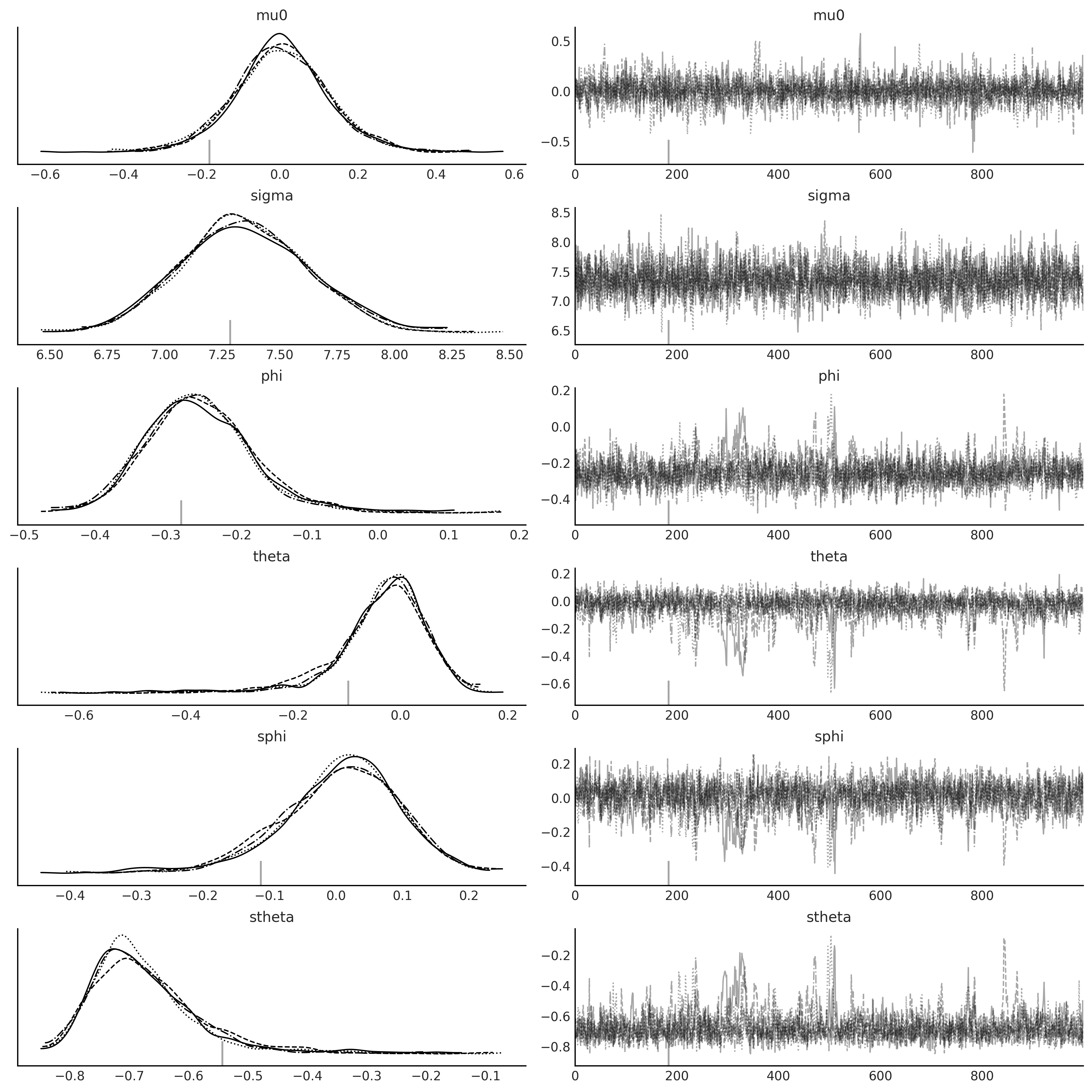
axes = az.plot_trace(nuts_trace_arima);

SARIMAX Class

import warnings
from statsmodels.tsa.statespace.tools import diff as tsa_diff
from tensorflow_probability.python.internal import distribution_util
from tensorflow_probability.python.internal import prefer_static as ps


class SARIMAX:
    # Similar to https://www.statsmodels.org/stable/generated/statsmodels.tsa.statespace.sarimax.SARIMAX.html
    # with simple differencing
    def __init__(self,
                 observed,
                 design_matrix=None,
                 order=(1, 0, 0),
                 seasonal_order=(0, 0, 0, 0),
                 dtype=np.float32
                 ):
        """
        SARIMAX Likelihood for univariate time series
        
        order - (p,d,q)
        seasonal_order - (P,D,Q,s)
        """
        # Static parameters
        self.p, self.d, self.q = order
        self.P, self.D, self.Q, self.period = seasonal_order

        # Dynamic regression
        if design_matrix is not None:
            assert ps.rank(design_matrix) >= 2
            assert ps.shape(design_matrix)[-2] == observed.shape[-1]

            # seasonal adjustment
            if self.period > 0:
                warnings.warn("""
                Can not model seasonal difference with Dynamic regressions,
                Setting D to 0 ...
                """)
                self.period = 0

            self.design_matrix = tf.convert_to_tensor(
                np.diff(design_matrix, n=self.d, axis=0), dtype=dtype)
        else:
            self.design_matrix = None

        if self.period <= 1:
            self.P, self.D, self.Q = 0, 0, 0

        self.r = max(self.p, self.q, self.P *
                     self.period, self.Q * self.period)

        # Simple differencing
        observed_diff = tsa_diff(
            observed,
            k_diff=self.d,
            k_seasonal_diff=self.D,
            seasonal_periods=self.period)
        self.observed = tf.convert_to_tensor(observed_diff, dtype=dtype)

        self.dtype = dtype

    def _log_prob(self, *args):
        mu0 = args[0]  # Location parameter
        sigma = args[1]  # Scale parameter
        i = 2
        if self.design_matrix is not None:  # regression coefficients
            reg_coeff = args[i]
            mu_t = mu0[None, ...] + \
                tf.einsum('...i,ji->j...', reg_coeff, self.design_matrix)
            i += 1
        else:
            mu_t = tf.einsum('...,j->j...', mu0, ps.ones_like(self.observed))

        # Parse args and prepare states
        if self.p > 0:  # AR coefficients
            phi = args[i]
            i += 1
        if self.q > 0:  # MA coefficients
            theta = args[i]
            i += 1
        if self.P > 0:  # SAR coefficients
            sphi = args[i]
            i += 1
        if self.Q > 0:  # SMA coefficients
            stheta = args[i]
            i += 1

        batch_shape = ps.shape(mu0)
        y_extended = ps.concat(
            [ps.zeros(tf.concat([[self.r], batch_shape], axis=0), dtype=mu0.dtype),
             tf.einsum('...,j->j...',
                       ps.ones_like(mu0, dtype=self.observed.dtype),
                       self.observed)],
            axis=0
        )
        eps_t = ps.zeros_like(y_extended, dtype=self.observed.dtype)

        def body_fn(t, mu_t, eps_t):
            mu_temp = []
            t_switch = t + self.r
            if self.p > 0:  # AR
                y_past = tf.gather(
                    y_extended, t_switch - (np.arange(self.p) + 1))
                ar = tf.einsum("...p,p...->...", phi, y_past)
                mu_temp.append(ar)
            if self.q > 0:  # MA
                eps_past = tf.gather(
                    eps_t, t_switch - (np.arange(self.q) + 1))
                ma = tf.einsum("...q,q...->...", theta, eps_past)
                mu_temp.append(ma)
            if self.P > 0:  # SAR
                y_past = tf.gather(
                    y_extended, t_switch - (np.arange(self.P) + 1) * self.period)
                sar = tf.einsum("...p,p...->...", sphi, y_past)
                mu_temp.append(sar)
            if self.Q > 0:  # SMA
                eps_past = tf.gather(
                    eps_t, t_switch - (np.arange(self.Q) + 1) * self.period)
                sma = tf.einsum("...q,q...->...", stheta, eps_past)
                mu_temp.append(sma)
            mu_update = sum(mu_temp) + tf.gather(mu_t, t)
            mu_t_next = tf.tensor_scatter_nd_update(
                mu_t, [[t]], mu_update[None, ...])

            eps_update = tf.gather(y_extended, t_switch) - mu_update
            epsilon_t_next = tf.tensor_scatter_nd_update(
                eps_t, [[t_switch]], eps_update[None, ...])
            return t+1, mu_t_next, epsilon_t_next

        t, mu_output, eps_output_ = tf.while_loop(
            lambda t, *_: t < self.observed.shape[-1],
            body_fn,
            loop_vars=(0, mu_t, eps_t),
            maximum_iterations=self.observed.shape[-1])
        eps_output = eps_output_[self.r:]
        return tfd.Normal(0, sigma[None, ...]).log_prob(eps_output), mu_output
    
    def log_prob(self, *args):
        log_prob_val, _ = self._log_prob(*args)
        return ps.reduce_sum(log_prob_val, axis=0)
    
    def log_prob_elementwise(self, *args):
        sigma = args[1]  # Scale parameter
        _, mu_output = self._log_prob(*args)
        mu = distribution_util.move_dimension(mu_output, 0, -1)
        return tfd.Normal(mu, sigma[..., None]).log_prob(self.observed)

y ~ Sarima(1,1,1)(1,1,1)[12]

p, q, P, Q = 1, 1, 1, 1

@tfd.JointDistributionCoroutine
def sarima_priors():
    mu0 = yield root(tfd.StudentT(df=6, loc=0, scale=2.5, name='mu0'))
    sigma = yield root(tfd.HalfStudentT(df=7, loc=0, scale=1., name='sigma'))

    phi = yield root(tfd.Sample(tfd.Normal(loc=0, scale=0.5), p, name='phi'))
    theta = yield root(tfd.Sample(tfd.Normal(loc=0, scale=0.5), q, name='theta'))
    sphi = yield root(tfd.Sample(tfd.Normal(loc=0, scale=0.5), P, name='sphi'))
    stheta = yield root(tfd.Sample(tfd.Normal(loc=0, scale=0.5), Q, name='stheta'))


sarima_1 = SARIMAX(
    us_monthly_birth["birth_in_thousands"],
    order=(1, 1, 1),
    seasonal_order=(1, 1, 1, 12))

%%time
target_log_prob_fn = lambda *x: sarima_priors.log_prob(
    *x) + sarima_1.log_prob(*x)

mcmc_samples, sampler_stats = run_mcmc_simple(
    1000, sarima_priors, n_chains=4, num_adaptation_steps=1000,
    target_log_prob_fn=target_log_prob_fn,
    seed=tf.constant([623453, 456345], dtype=tf.int32),
)

WARNING:tensorflow:@custom_gradient grad_fn has 'variables' in signature, but no ResourceVariables were used on the forward pass.
WARNING:tensorflow:@custom_gradient grad_fn has 'variables' in signature, but no ResourceVariables were used on the forward pass.
WARNING:tensorflow:@custom_gradient grad_fn has 'variables' in signature, but no ResourceVariables were used on the forward pass.
WARNING:tensorflow:@custom_gradient grad_fn has 'variables' in signature, but no ResourceVariables were used on the forward pass.
WARNING:tensorflow:@custom_gradient grad_fn has 'variables' in signature, but no ResourceVariables were used on the forward pass.
WARNING:tensorflow:@custom_gradient grad_fn has 'variables' in signature, but no ResourceVariables were used on the forward pass.
WARNING:tensorflow:@custom_gradient grad_fn has 'variables' in signature, but no ResourceVariables were used on the forward pass.
WARNING:tensorflow:@custom_gradient grad_fn has 'variables' in signature, but no ResourceVariables were used on the forward pass.
WARNING:tensorflow:@custom_gradient grad_fn has 'variables' in signature, but no ResourceVariables were used on the forward pass.
WARNING:tensorflow:@custom_gradient grad_fn has 'variables' in signature, but no ResourceVariables were used on the forward pass.
CPU times: user 30.5 s, sys: 479 ms, total: 31 s
Wall time: 31.1 s

data_likelihood = np.swapaxes(sarima_1.log_prob_elementwise(*mcmc_samples), 1, 0)
sarima_0_idata = az.from_dict(
    posterior={
        k:np.swapaxes(v.numpy(), 1, 0)
        for k, v in mcmc_samples._asdict().items()},
    sample_stats={
        k:np.swapaxes(sampler_stats[k], 1, 0)
        for k in ["target_log_prob", "diverging", "accept_ratio", "n_steps"]},
    observed_data={'observed': sarima_1.observed},
    log_likelihood={'observed': data_likelihood},
)

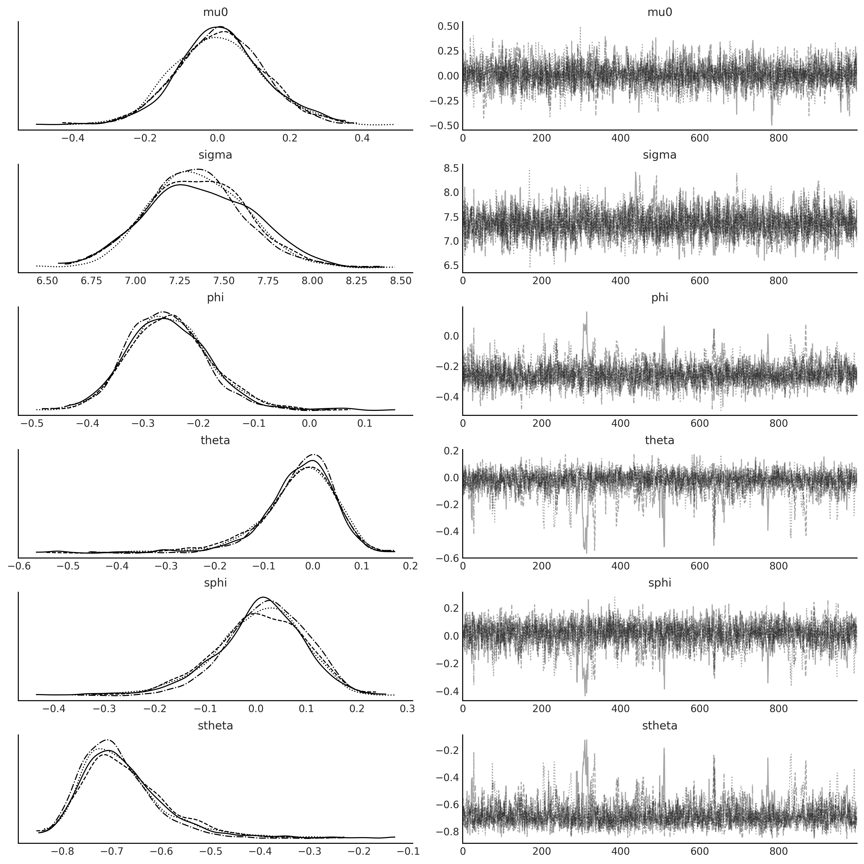
axes = az.plot_trace(sarima_0_idata);

Code 6.8

def gen_fourier_basis(t, p=365.25, n=3):
    x = 2 * np.pi * (np.arange(n) + 1) * t[:, None] / p
    return np.concatenate((np.cos(x), np.sin(x)), axis=1)


p = 12
t_monthly = np.asarray([i % p for i in range(len(us_monthly_birth))]) + 1
monthly_X = gen_fourier_basis(t_monthly, p=p, n=2)


@tfd.JointDistributionCoroutine
def sarima_priors():
    mu0 = yield root(tfd.StudentT(df=6, loc=0, scale=2.5, name='mu0'))
    sigma = yield root(tfd.HalfStudentT(df=7, loc=0, scale=1., name='sigma'))
    beta = yield root(tfd.Sample(
        tfd.StudentT(df=6, loc=0, scale=2.5),
        monthly_X.shape[-1],
        name='beta'))
    phi = yield root(tfd.Sample(tfd.Normal(loc=0, scale=0.5), 1, name='phi'))
    theta = yield root(tfd.Sample(tfd.Normal(loc=0, scale=0.5), 1, name='theta'))


sarima_2 = SARIMAX(
    us_monthly_birth["birth_in_thousands"],
    design_matrix=monthly_X,
    order=(1, 1, 1))

%%time
target_log_prob_fn = lambda *x: sarima_priors.log_prob(
    *x) + sarima_2.log_prob(*x)

mcmc_samples, sampler_stats = run_mcmc_simple(
    1000, sarima_priors, n_chains=4, num_adaptation_steps=1000,
    target_log_prob_fn=target_log_prob_fn,
    seed=tf.constant([623453, 456345], dtype=tf.int32),
)

WARNING:tensorflow:@custom_gradient grad_fn has 'variables' in signature, but no ResourceVariables were used on the forward pass.
WARNING:tensorflow:@custom_gradient grad_fn has 'variables' in signature, but no ResourceVariables were used on the forward pass.
WARNING:tensorflow:@custom_gradient grad_fn has 'variables' in signature, but no ResourceVariables were used on the forward pass.
WARNING:tensorflow:@custom_gradient grad_fn has 'variables' in signature, but no ResourceVariables were used on the forward pass.
WARNING:tensorflow:@custom_gradient grad_fn has 'variables' in signature, but no ResourceVariables were used on the forward pass.
WARNING:tensorflow:@custom_gradient grad_fn has 'variables' in signature, but no ResourceVariables were used on the forward pass.
WARNING:tensorflow:@custom_gradient grad_fn has 'variables' in signature, but no ResourceVariables were used on the forward pass.
WARNING:tensorflow:@custom_gradient grad_fn has 'variables' in signature, but no ResourceVariables were used on the forward pass.
WARNING:tensorflow:@custom_gradient grad_fn has 'variables' in signature, but no ResourceVariables were used on the forward pass.
WARNING:tensorflow:@custom_gradient grad_fn has 'variables' in signature, but no ResourceVariables were used on the forward pass.
WARNING:tensorflow:@custom_gradient grad_fn has 'variables' in signature, but no ResourceVariables were used on the forward pass.
WARNING:tensorflow:@custom_gradient grad_fn has 'variables' in signature, but no ResourceVariables were used on the forward pass.
WARNING:tensorflow:@custom_gradient grad_fn has 'variables' in signature, but no ResourceVariables were used on the forward pass.
WARNING:tensorflow:@custom_gradient grad_fn has 'variables' in signature, but no ResourceVariables were used on the forward pass.
WARNING:tensorflow:@custom_gradient grad_fn has 'variables' in signature, but no ResourceVariables were used on the forward pass.
CPU times: user 33.9 s, sys: 598 ms, total: 34.5 s
Wall time: 34.6 s

data_likelihood = np.swapaxes(sarima_2.log_prob_elementwise(*mcmc_samples), 1, 0)
arimax_idata = az.from_dict(
    posterior={
        k:np.swapaxes(v.numpy(), 1, 0)
        for k, v in mcmc_samples._asdict().items()},
    sample_stats={
        k:np.swapaxes(sampler_stats[k], 1, 0)
        for k in ["target_log_prob", "diverging", "accept_ratio", "n_steps"]},
    observed_data={'observed': sarima_2.observed},
    log_likelihood={'observed': data_likelihood},
)

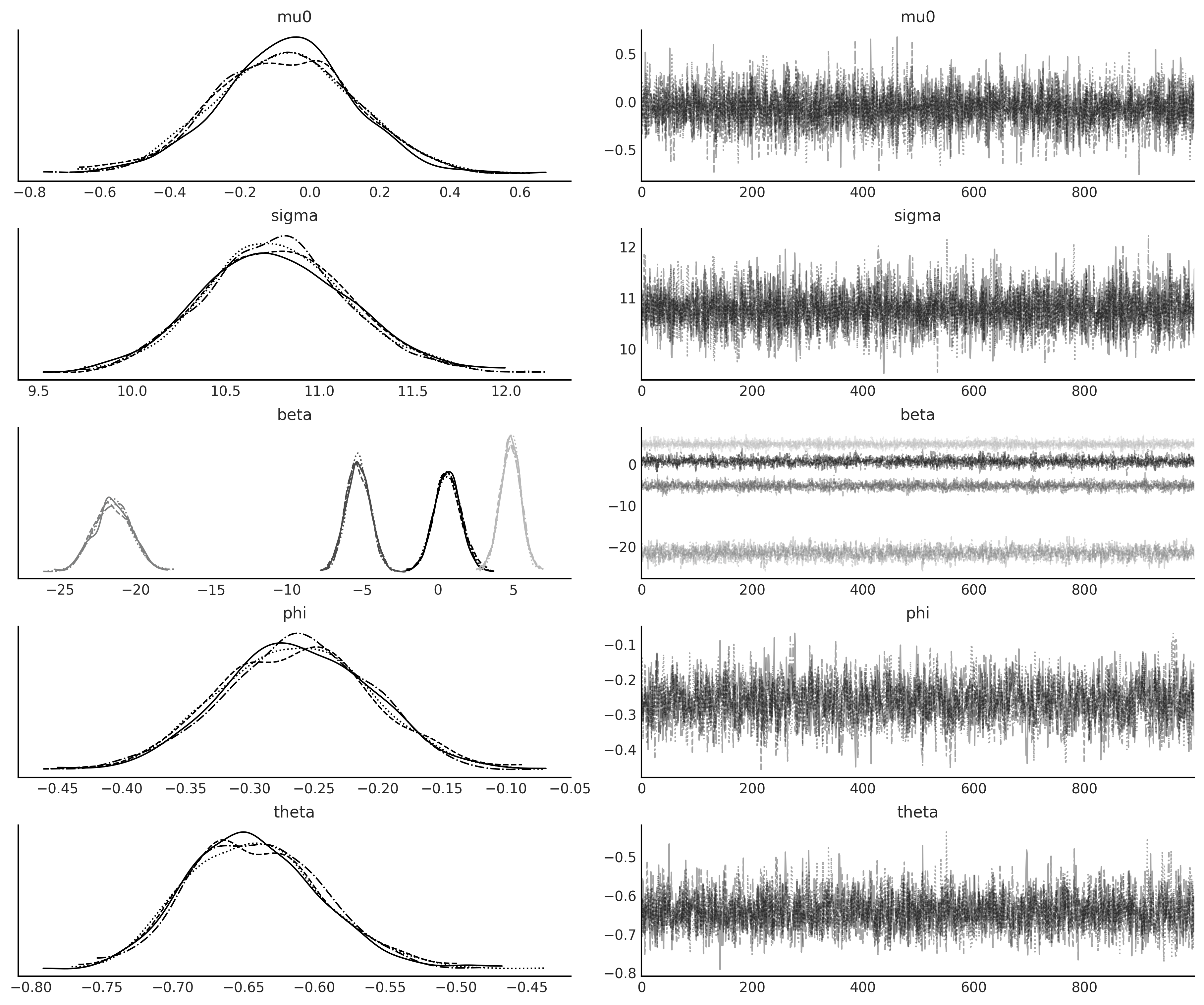
axes = az.plot_trace(arimax_idata);

y ~ Sarima(0,1,2)(1,1,1)[12]

@tfd.JointDistributionCoroutine
def sarima_priors():
    mu0 = yield root(tfd.StudentT(df=6, loc=0, scale=2.5, name='mu0'))
    sigma = yield root(tfd.HalfStudentT(df=7, loc=0, scale=1., name='sigma'))

    theta = yield root(tfd.Sample(tfd.Normal(loc=0, scale=0.5), 2, name='theta'))
    sphi = yield root(tfd.Sample(tfd.Normal(loc=0, scale=0.5), 1, name='sphi'))
    stheta = yield root(tfd.Sample(tfd.Normal(loc=0, scale=0.5), 1, name='stheta'))

sarima_3 = SARIMAX(
    us_monthly_birth["birth_in_thousands"],
    order=(0, 1, 2),
    seasonal_order=(1, 1, 1, 12))

%%time
target_log_prob_fn = lambda *x: sarima_priors.log_prob(
    *x) + sarima_3.log_prob(*x)

mcmc_samples, sampler_stats = run_mcmc_simple(
    1000, sarima_priors, n_chains=4, num_adaptation_steps=1000,
    target_log_prob_fn=target_log_prob_fn,
    seed=tf.constant([934563, 12356], dtype=tf.int32),
)

WARNING:tensorflow:@custom_gradient grad_fn has 'variables' in signature, but no ResourceVariables were used on the forward pass.
WARNING:tensorflow:@custom_gradient grad_fn has 'variables' in signature, but no ResourceVariables were used on the forward pass.
WARNING:tensorflow:@custom_gradient grad_fn has 'variables' in signature, but no ResourceVariables were used on the forward pass.
WARNING:tensorflow:@custom_gradient grad_fn has 'variables' in signature, but no ResourceVariables were used on the forward pass.
WARNING:tensorflow:@custom_gradient grad_fn has 'variables' in signature, but no ResourceVariables were used on the forward pass.
WARNING:tensorflow:@custom_gradient grad_fn has 'variables' in signature, but no ResourceVariables were used on the forward pass.
WARNING:tensorflow:@custom_gradient grad_fn has 'variables' in signature, but no ResourceVariables were used on the forward pass.
WARNING:tensorflow:@custom_gradient grad_fn has 'variables' in signature, but no ResourceVariables were used on the forward pass.
WARNING:tensorflow:@custom_gradient grad_fn has 'variables' in signature, but no ResourceVariables were used on the forward pass.
WARNING:tensorflow:@custom_gradient grad_fn has 'variables' in signature, but no ResourceVariables were used on the forward pass.
CPU times: user 1min 2s, sys: 812 ms, total: 1min 3s
Wall time: 1min 3s

data_likelihood = np.swapaxes(sarima_3.log_prob_elementwise(*mcmc_samples), 1, 0)
sarima_1_idata = az.from_dict(
    posterior={
        k:np.swapaxes(v.numpy(), 1, 0)
        for k, v in mcmc_samples._asdict().items()},
    sample_stats={
        k:np.swapaxes(sampler_stats[k], 1, 0)
        for k in ["target_log_prob", "diverging", "accept_ratio", "n_steps"]},
    observed_data={'observed': sarima_2.observed},
    log_likelihood={'observed': data_likelihood},
)

axes = az.plot_trace(sarima_1_idata);

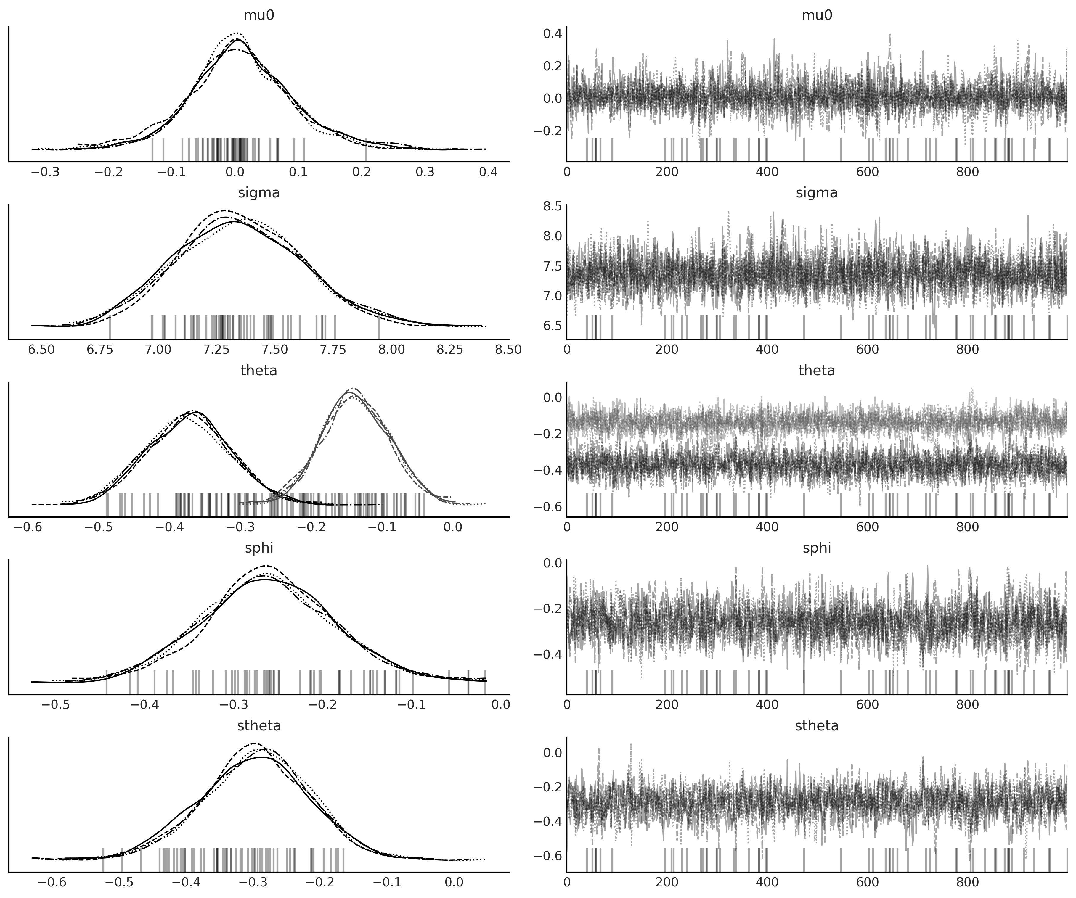
az.summary(sarima_1_idata)

	mean	sd	hdi_3%	hdi_97%	mcse_mean	mcse_sd	ess_bulk	ess_tail	r_hat
mu0	0.010	0.084	-0.148	0.179	0.002	0.001	2648.0	2030.0	1.0
sigma	7.354	0.277	6.820	7.863	0.005	0.004	3004.0	2521.0	1.0
theta[0]	-0.373	0.060	-0.489	-0.265	0.001	0.001	2359.0	2522.0	1.0
theta[1]	-0.137	0.048	-0.226	-0.046	0.001	0.001	2644.0	2533.0	1.0
sphi[0]	-0.261	0.075	-0.404	-0.123	0.002	0.001	1731.0	2276.0	1.0
stheta[0]	-0.297	0.082	-0.454	-0.148	0.002	0.002	1561.0	2073.0	1.0

Table 6.1

compare_dict = {"SARIMA(1,1,1)(1,1,1)[12]": sarima_0_idata,
#                 "ARIMAX(1,1,1)X[4]": arimax_idata,
                "SARIMA(0,1,2)(1,1,1)[12]": sarima_1_idata}
cmp = az.compare(compare_dict, ic='loo')
cmp.round(2)

/opt/miniconda3/envs/bmcp/lib/python3.9/site-packages/arviz/stats/stats.py:145: UserWarning: The default method used to estimate the weights for each model,has changed from BB-pseudo-BMA to stacking
  warnings.warn(

	rank	loo	p_loo	d_loo	weight	se	dse	warning	loo_scale
SARIMA(1,1,1)(1,1,1)[12]	0	-1235.61	7.73	0.00	0.51	15.46	0.00	False	log
SARIMA(0,1,2)(1,1,1)[12]	1	-1235.62	7.49	0.01	0.49	15.39	6.35	False	log

# print(cmp.round(2).to_latex())

State Space Models

Code 6.19

theta0, theta1 = 1.2, 2.6
sigma = 0.4
num_timesteps = 100

time_stamp = tf.linspace(0., 1., num_timesteps)[..., None]
yhat = theta0 + theta1 * time_stamp
y = tfd.Normal(yhat, sigma).sample()

Code 6.20

# X_0
initial_state_prior = tfd.MultivariateNormalDiag(
    loc=[0., 0.], scale_diag=[5., 5.])
# F_t
transition_matrix = lambda _: tf.linalg.LinearOperatorIdentity(2)
# eta_t ~ Normal(0, Q_t)
transition_noise = lambda _: tfd.MultivariateNormalDiag(
    loc=[0., 0.], scale_diag=[0., 0.])
# H_t
H = tf.concat([tf.ones_like(time_stamp), time_stamp], axis=-1)
observation_matrix = lambda t: tf.linalg.LinearOperatorFullMatrix(
    [tf.gather(H, t)])
# epsilon_t ~ Normal(0, R_t)
observation_noise = lambda _: tfd.MultivariateNormalDiag(
    loc=[0.], scale_diag=[sigma])

linear_growth_model = tfd.LinearGaussianStateSpaceModel(
    num_timesteps=num_timesteps,
    transition_matrix=transition_matrix,
    transition_noise=transition_noise,
    observation_matrix=observation_matrix,
    observation_noise=observation_noise,
    initial_state_prior=initial_state_prior)

Code 6.21

# Run the Kalman filter
(
    log_likelihoods,
    mt_filtered, Pt_filtered,
    mt_predicted, Pt_predicted,
    observation_means, observation_cov  # observation_cov is S_t
) = linear_growth_model.forward_filter(y)

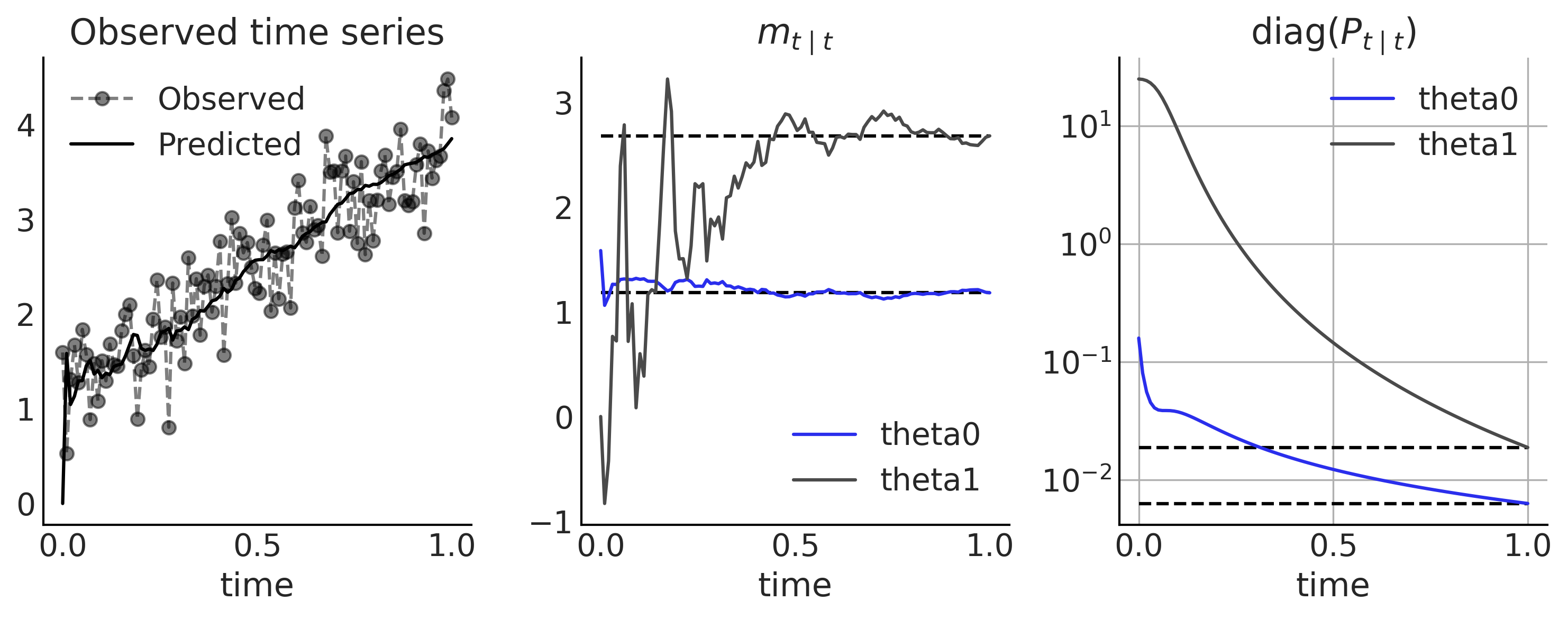
Figure 6.16

m0 = initial_state_prior.mean()
P0 = initial_state_prior.covariance()

P0_inv = tf.linalg.inv(P0)
P_t = tf.linalg.inv(P0_inv + 
                    1 / sigma **2 * (tf.matmul(H, H, transpose_a=True)))
m_t = tf.matmul(P_t, (1 / sigma **2 * (tf.matmul(H, y, transpose_a=True)) + 
                      tf.matmul(P0_inv, m0[..., None])))
filtered_vars = tf.linalg.diag_part(Pt_filtered)

_, ax = plt.subplots(1, 3, figsize=(10, 4))
ax[0].plot(time_stamp, y, '--o', alpha=.5);
ax[0].plot(time_stamp, observation_means, lw=1.5, color='k')
ax[0].set_title('Observed time series')
ax[0].legend(['Observed', 'Predicted'])
ax[0].set_xlabel('time');

color = ['C4', 'C1']
for i in range(2):
    ax[1].plot(time_stamp, tf.transpose(mt_filtered[..., i]), color=color[i]);
    ax[2].semilogy(time_stamp, tf.transpose(filtered_vars[..., i]), color=color[i]);
for i in range(2):
    ax[i+1].set_xlabel('time')
    ax[i+1].legend(['theta0', 'theta1'])

ax[1].hlines(m_t, time_stamp[0], time_stamp[-1], ls='--');
ax[1].set_title(r'$m_{t \mid t}$')
ax[2].hlines(tf.linalg.diag_part(P_t), time_stamp[0], time_stamp[-1], ls='--')
ax[2].set_title(r'diag($P_{t \mid t}$)')
ax[2].grid()
plt.tight_layout();

plt.savefig("img/chp06/fig16_linear_growth_lgssm.png");

/var/folders/7p/srk5qjp563l5f9mrjtp44bh800jqsw/T/ipykernel_14469/3981273553.py:31: UserWarning: This figure was using constrained_layout, but that is incompatible with subplots_adjust and/or tight_layout; disabling constrained_layout.
  plt.tight_layout();

ARMA as LGSSM

Code 6.22

num_timesteps = 300
phi1 = -.1
phi2 = .5
theta1 = -.25
sigma = 1.25

# X_0
initial_state_prior = tfd.MultivariateNormalDiag(
    scale_diag=[sigma, sigma])
# F_t
transition_matrix = lambda _: tf.linalg.LinearOperatorFullMatrix(
    [[phi1, 1], [phi2, 0]])
# eta_t ~ Normal(0, Q_t)
R_t = tf.constant([[sigma], [sigma*theta1]])
Q_t_tril = tf.concat([R_t, tf.zeros_like(R_t)], axis=-1)
transition_noise = lambda _: tfd.MultivariateNormalTriL(
    scale_tril=Q_t_tril)
# H_t
observation_matrix = lambda t: tf.linalg.LinearOperatorFullMatrix(
    [[1., 0.]])
# epsilon_t ~ Normal(0, 0)
observation_noise = lambda _: tfd.MultivariateNormalDiag(
    loc=[0.], scale_diag=[0.])

arma = tfd.LinearGaussianStateSpaceModel(
    num_timesteps=num_timesteps,
    transition_matrix=transition_matrix,
    transition_noise=transition_noise,
    observation_matrix=observation_matrix,
    observation_noise=observation_noise,
    initial_state_prior=initial_state_prior
    )

# Simulate from the model
sim_ts = arma.sample()

np.linalg.eigvals(Q_t_tril @ tf.transpose(Q_t_tril)) >= 0

array([ True,  True])

plt.plot(sim_ts);

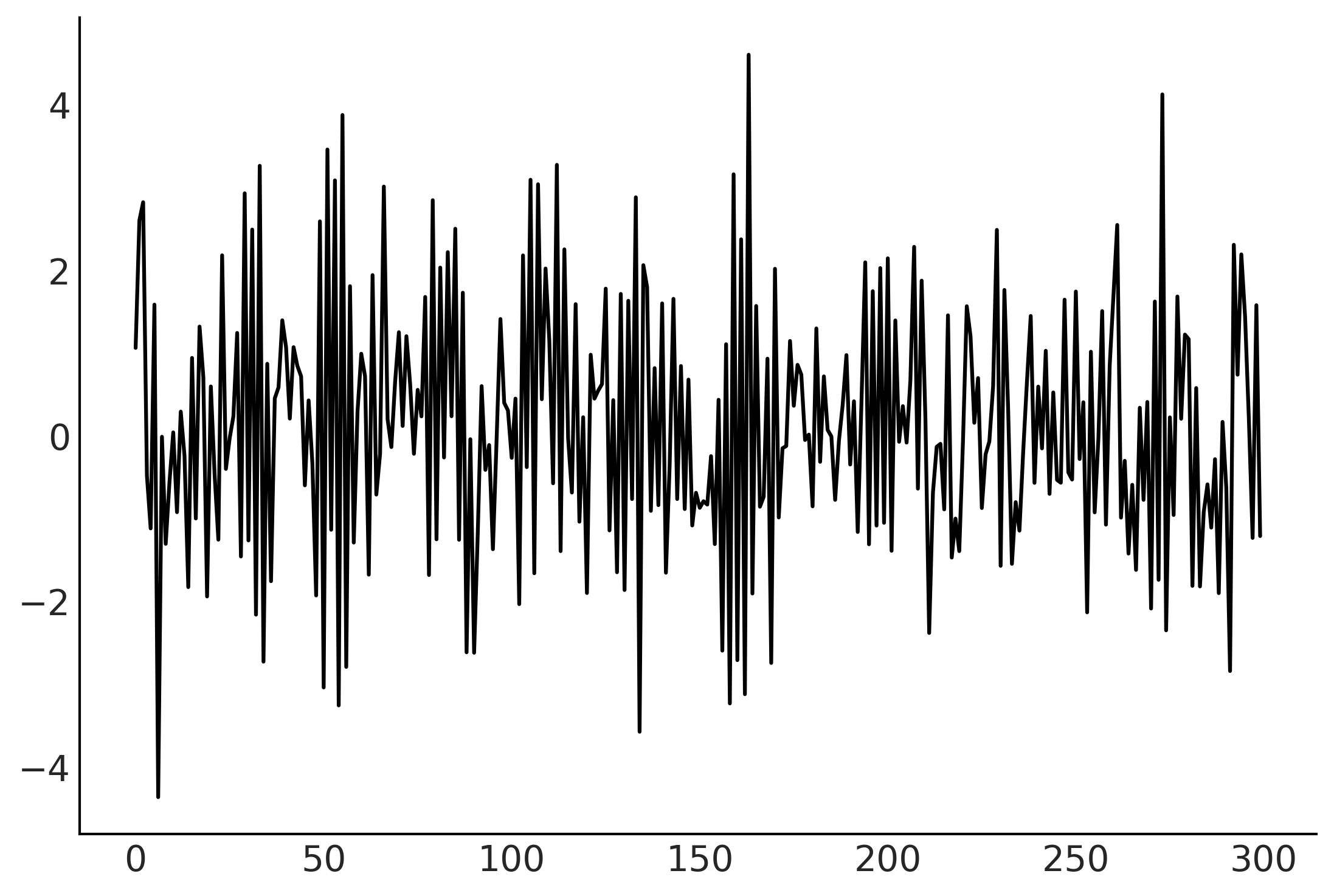
arma.log_prob(sim_ts)

<tf.Tensor: shape=(), dtype=float32, numpy=-492.00345>

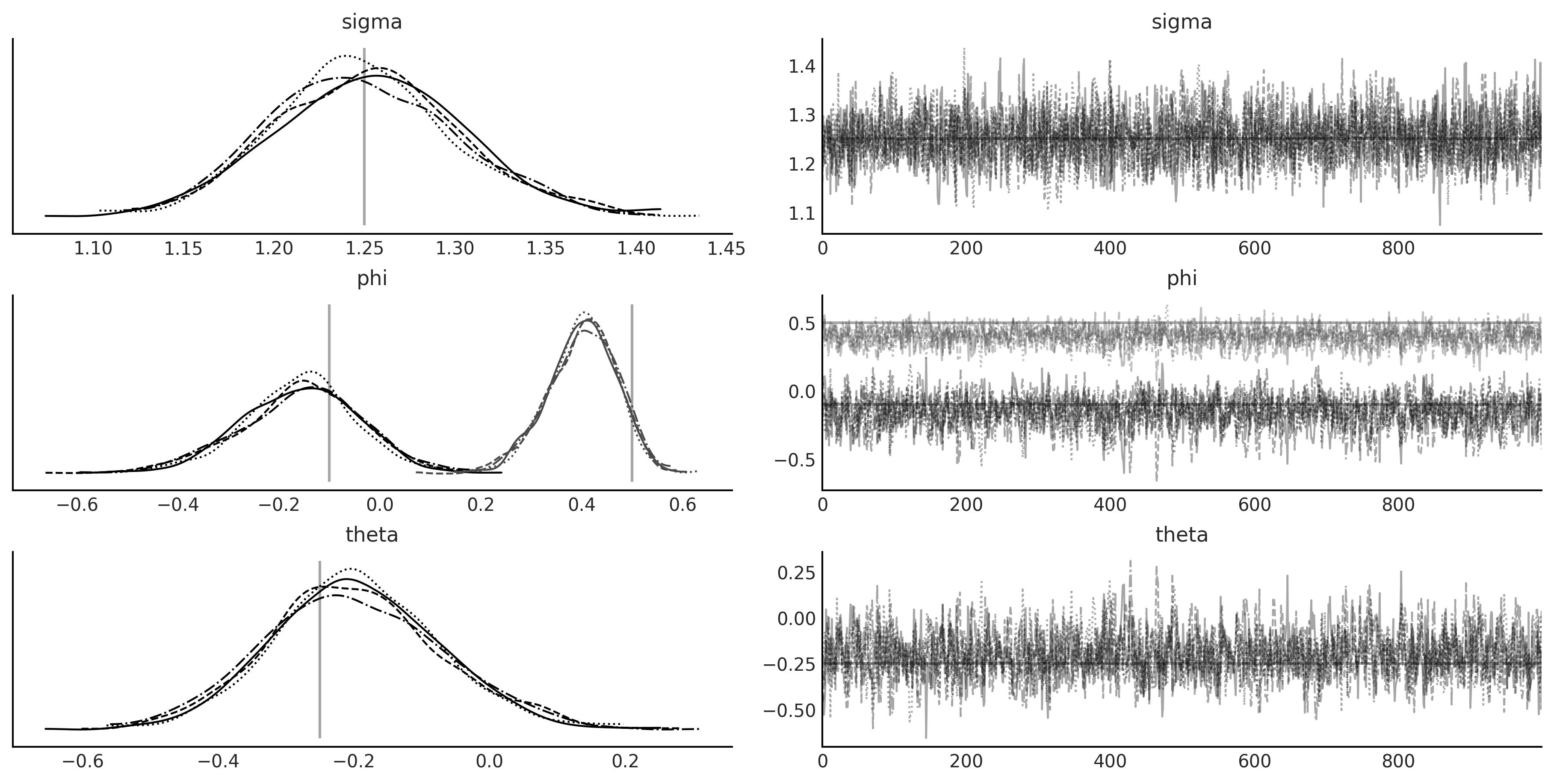
Code 6.23

@tfd.JointDistributionCoroutine
def arma_lgssm():
    sigma = yield root(tfd.HalfStudentT(df=7, loc=0, scale=1., name='sigma'))
    phi = yield root(tfd.Sample(tfd.Normal(loc=0, scale=0.5), 2, name='phi'))
    theta = yield root(tfd.Sample(tfd.Normal(loc=0, scale=0.5), 1, name='theta'))

    # X0
    init_scale_diag = tf.concat([sigma[..., None], sigma[..., None]], axis=-1)
    initial_state_prior = tfd.MultivariateNormalDiag(
        scale_diag=init_scale_diag)

    F_t = tf.concat([phi[..., None],
                     tf.concat([tf.ones_like(phi[..., 0, None]),
                                tf.zeros_like(phi[..., 0, None])],
                               axis=-1)[..., None]],
                    axis=-1)

    def transition_matrix(_): return tf.linalg.LinearOperatorFullMatrix(F_t)

    transition_scale_tril = tf.concat(
        [sigma[..., None], theta * sigma[..., None]], axis=-1)[..., None]
    scale_tril = tf.concat(
        [transition_scale_tril,
         tf.zeros_like(transition_scale_tril)],
        axis=-1)

    def transition_noise(_): return tfd.MultivariateNormalTriL(
        scale_tril=scale_tril)

    def observation_matrix(
        t): return tf.linalg.LinearOperatorFullMatrix([[1., 0.]])

    def observation_noise(t): return tfd.MultivariateNormalDiag(
        loc=[0], scale_diag=[0.])

    arma = yield tfd.LinearGaussianStateSpaceModel(
        num_timesteps=num_timesteps,
        transition_matrix=transition_matrix,
        transition_noise=transition_noise,
        observation_matrix=observation_matrix,
        observation_noise=observation_noise,
        initial_state_prior=initial_state_prior,
        name='arma')

%%time
mcmc_samples, sampler_stats = run_mcmc_simple(
    1000, arma_lgssm, n_chains=4, num_adaptation_steps=1000,
    seed=tf.constant([23453, 94567], dtype=tf.int32),
    arma=sim_ts)

WARNING:tensorflow:@custom_gradient grad_fn has 'variables' in signature, but no ResourceVariables were used on the forward pass.
WARNING:tensorflow:@custom_gradient grad_fn has 'variables' in signature, but no ResourceVariables were used on the forward pass.
WARNING:tensorflow:@custom_gradient grad_fn has 'variables' in signature, but no ResourceVariables were used on the forward pass.
WARNING:tensorflow:@custom_gradient grad_fn has 'variables' in signature, but no ResourceVariables were used on the forward pass.
WARNING:tensorflow:@custom_gradient grad_fn has 'variables' in signature, but no ResourceVariables were used on the forward pass.
WARNING:tensorflow:5 out of the last 5 calls to <function run_mcmc_simple.<locals>.run_inference_nuts at 0x7fad6303a700> triggered tf.function retracing. Tracing is expensive and the excessive number of tracings could be due to (1) creating @tf.function repeatedly in a loop, (2) passing tensors with different shapes, (3) passing Python objects instead of tensors. For (1), please define your @tf.function outside of the loop. For (2), @tf.function has experimental_relax_shapes=True option that relaxes argument shapes that can avoid unnecessary retracing. For (3), please refer to https://www.tensorflow.org/guide/function#controlling_retracing and https://www.tensorflow.org/api_docs/python/tf/function for  more details.
CPU times: user 29.2 s, sys: 476 ms, total: 29.7 s
Wall time: 29.8 s

Figure 6.17

test_trace = az.from_dict(
    posterior={
        k:np.swapaxes(v.numpy(), 1, 0)
        for k, v in mcmc_samples._asdict().items()},
    sample_stats={
        k:np.swapaxes(sampler_stats[k], 1, 0)
        for k in ["target_log_prob", "diverging", "accept_ratio", "n_steps"]}
)

lines = (('sigma', {}, sigma), ('phi', {}, [phi1, phi2]), ('theta', {}, theta1),)
axes = az.plot_trace(test_trace, lines=lines);

plt.savefig("img/chp06/fig17_arma_lgssm_inference_result.png");

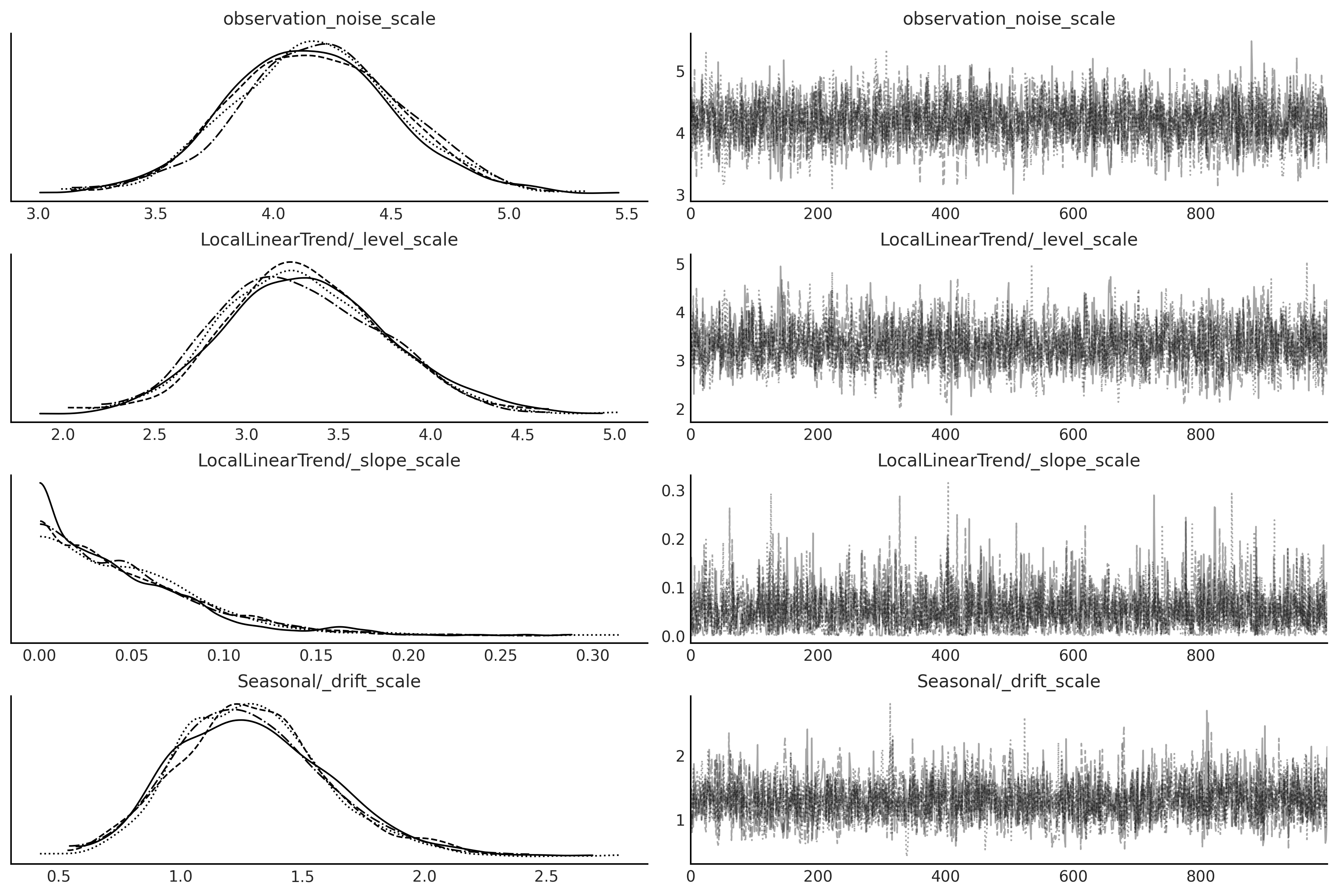
Bayesian Structural Time Series Models on Monthly Live Birth Data

def generate_bsts_model(observed=None):
    """
    Args:
    observed: Observed time series, tfp.sts use it to generate data informed prior.
    """
    # Trend
    trend = tfp.sts.LocalLinearTrend(observed_time_series=observed)
    # Seasonal
    seasonal = tfp.sts.Seasonal(num_seasons=12, observed_time_series=observed)
    # Full model
    return tfp.sts.Sum([trend, seasonal], observed_time_series=observed)

observed = tf.constant(us_monthly_birth["birth_in_thousands"], dtype=tf.float32)
birth_model = generate_bsts_model(observed=observed)

# Generate the posterior distribution conditioned on the observed
# target_log_prob_fn = birth_model.joint_log_prob(observed_time_series=observed)

birth_model_jd = birth_model.joint_distribution(observed_time_series=observed)

WARNING:tensorflow:From /opt/miniconda3/envs/bmcp/lib/python3.9/site-packages/tensorflow/python/ops/linalg/linear_operator_composition.py:182: LinearOperator.graph_parents (from tensorflow.python.ops.linalg.linear_operator) is deprecated and will be removed in a future version.
Instructions for updating:
Do not call `graph_parents`.
WARNING:tensorflow:From /opt/miniconda3/envs/bmcp/lib/python3.9/site-packages/tensorflow_probability/python/distributions/distribution.py:342: MultivariateNormalFullCovariance.__init__ (from tensorflow_probability.python.distributions.mvn_full_covariance) is deprecated and will be removed after 2019-12-01.
Instructions for updating:
`MultivariateNormalFullCovariance` is deprecated, use `MultivariateNormalTriL(loc=loc, scale_tril=tf.linalg.cholesky(covariance_matrix))` instead.

Code 6.25

birth_model.components

[<tensorflow_probability.python.sts.components.local_linear_trend.LocalLinearTrend at 0x7fae436e6cd0>,
 <tensorflow_probability.python.sts.components.seasonal.Seasonal at 0x7fae76b00340>]

Code 6.26

birth_model.components[1].parameters

[Parameter(name='drift_scale', prior=<tfp.distributions.LogNormal 'LogNormal' batch_shape=[] event_shape=[] dtype=float32>, bijector=<tfp.bijectors.Chain 'chain_of_scale_of_softplus' batch_shape=[] forward_min_event_ndims=0 inverse_min_event_ndims=0 dtype_x=float32 dtype_y=float32 bijectors=[<tfp.bijectors.Scale 'scale' batch_shape=[] forward_min_event_ndims=0 inverse_min_event_ndims=0 dtype_x=float32 dtype_y=float32>, <tfp.bijectors.Softplus 'softplus' batch_shape=[] forward_min_event_ndims=0 inverse_min_event_ndims=0 dtype_x=float32 dtype_y=float32>]>)]

%%time
mcmc_samples, sampler_stats = run_mcmc(
    1000, birth_model_jd, n_chains=4, num_adaptation_steps=1000,
    seed=tf.constant([745678, 562345], dtype=tf.int32))

2021-11-19 18:01:06.021471: W tensorflow/compiler/tf2xla/kernels/assert_op.cc:38] Ignoring Assert operator mcmc_retry_init/assert_equal_1/Assert/AssertGuard/Assert

WARNING:tensorflow:6 out of the last 10 calls to <function windowed_adaptive_nuts at 0x7fae934af550> triggered tf.function retracing. Tracing is expensive and the excessive number of tracings could be due to (1) creating @tf.function repeatedly in a loop, (2) passing tensors with different shapes, (3) passing Python objects instead of tensors. For (1), please define your @tf.function outside of the loop. For (2), @tf.function has experimental_relax_shapes=True option that relaxes argument shapes that can avoid unnecessary retracing. For (3), please refer to https://www.tensorflow.org/guide/function#controlling_retracing and https://www.tensorflow.org/api_docs/python/tf/function for  more details.
CPU times: user 11min 21s, sys: 7.45 s, total: 11min 29s
Wall time: 11min 22s

birth_model_idata = az.from_dict(
    posterior={
        k:np.swapaxes(v.numpy(), 1, 0)
        for k, v in mcmc_samples.items()},
    sample_stats={
        k:np.swapaxes(sampler_stats[k], 1, 0)
        for k in ["target_log_prob", "diverging", "accept_ratio", "n_steps"]}
)

axes = az.plot_trace(birth_model_idata);

Code 6.27

# Using a subset of posterior samples.
parameter_samples = tf.nest.map_structure(lambda x: x[-100:, 0, ...], mcmc_samples)

# Get structual compoenent.
component_dists = tfp.sts.decompose_by_component(
    birth_model,
    observed_time_series=observed,
    parameter_samples=parameter_samples)

# Get forecast for n_steps.
n_steps = 36
forecast_dist = tfp.sts.forecast(
    birth_model,
    observed_time_series=observed,
    parameter_samples=parameter_samples,
    num_steps_forecast=n_steps)

Other Time Series Models

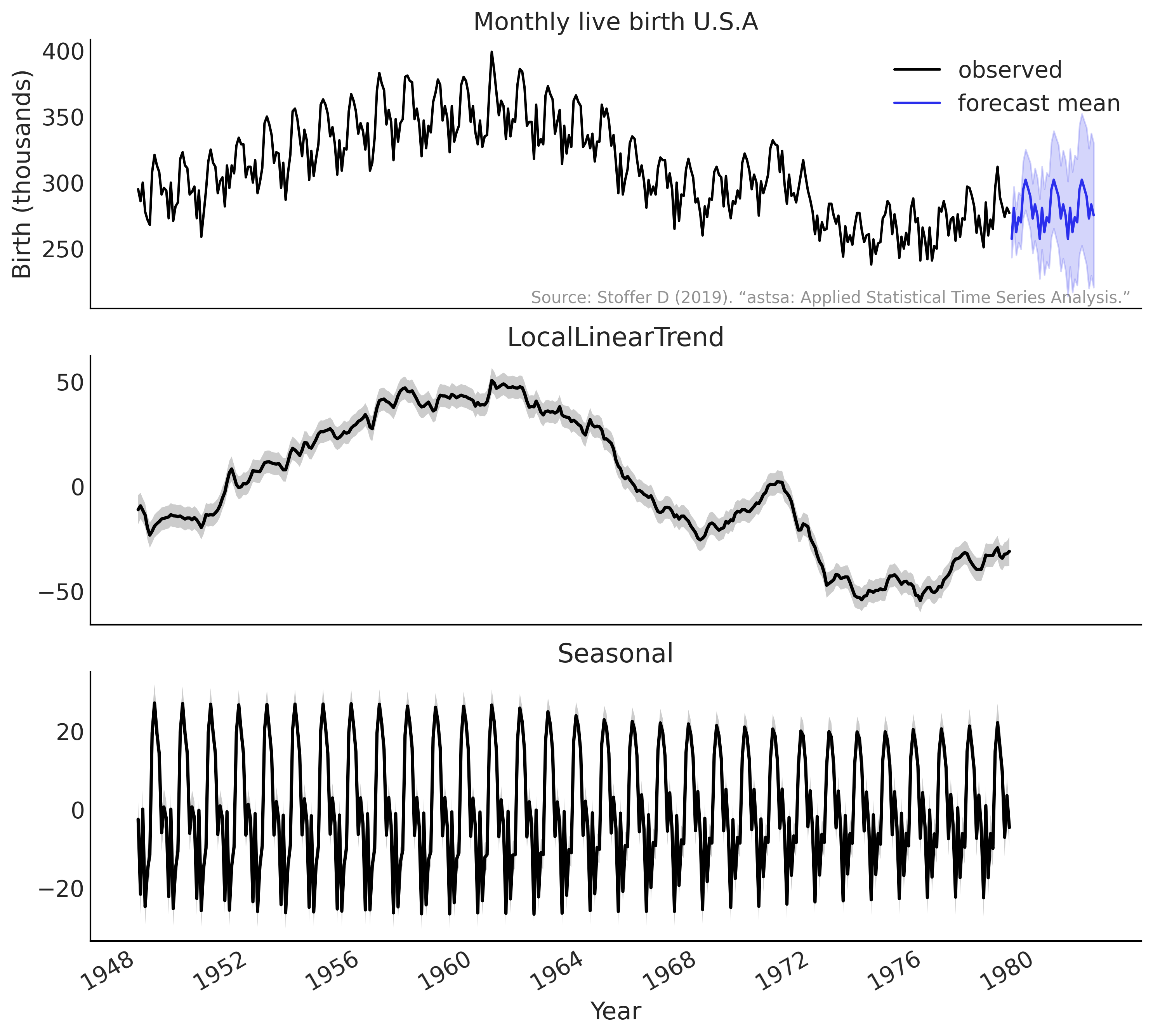
Figure 6.19

birth_dates = us_monthly_birth.index
forecast_date = pd.date_range(
    start=birth_dates[-1] + np.timedelta64(1, "M"),
    end=birth_dates[-1] + np.timedelta64(1 + n_steps, "M"),
    freq='M')

fig, axes = plt.subplots(
    1 + len(component_dists.keys()), 1, figsize=(10, 9), sharex=True)

ax = axes[0]
ax.plot(us_monthly_birth, lw=1.5, label='observed')

forecast_mean = np.squeeze(forecast_dist.mean())
line = ax.plot(forecast_date, forecast_mean, lw=1.5,
               label='forecast mean', color='C4')

forecast_std = np.squeeze(forecast_dist.stddev())
ax.fill_between(forecast_date,
                forecast_mean - 2 * forecast_std,
                forecast_mean + 2 * forecast_std,
                color=line[0].get_color(), alpha=0.2)

for ax_, (key, dist) in zip(axes[1:], component_dists.items()):
    comp_mean, comp_std = np.squeeze(dist.mean()), np.squeeze(dist.stddev())
    line = ax_.plot(birth_dates, dist.mean(), lw=2.)
    ax_.fill_between(birth_dates,
                     comp_mean - 2 * comp_std,
                     comp_mean + 2 * comp_std,
                     alpha=0.2)
    ax_.set_title(key.name[:-1])

ax.legend()

ax.set_ylabel("Birth (thousands)")
ax_.set_xlabel("Year")
ax.set_title("Monthly live birth U.S.A", fontsize=15)
ax.text(0.99, .02,
        "Source: Stoffer D (2019). “astsa: Applied Statistical Time Series Analysis.”",
        transform=ax.transAxes,
        horizontalalignment="right",
        alpha=0.5)

fig.autofmt_xdate()
plt.tight_layout()

plt.savefig("img/chp06/fig19_bsts_lgssm_result.png")

/var/folders/7p/srk5qjp563l5f9mrjtp44bh800jqsw/T/ipykernel_14469/2909654341.py:43: UserWarning: This figure was using constrained_layout, but that is incompatible with subplots_adjust and/or tight_layout; disabling constrained_layout.
  fig.autofmt_xdate()