5. Splines#
In this chapter we will discuss splines, which is an extension of concepts introduced into Chapter 3 with the aim of adding more flexibility. In the models introduced in Chapter 3 the relationship between the dependent and independent variables was the same for their entire domain. Splines, in contrast, can split a problem into multiple local solutions, which can all be combined to produce a useful global solution. Let us see how.
5.1. Polynomial Regression#
As we already saw in Chapter 3, we can write a linear model as:
where \(\beta_0\) is the intercept, \(\beta_1\) the slope and \(\mathbb{E}[Y]\) is the expected value, or mean, of the response (random) variable \(Y\). We can rewrite Equation (5.1) into the following form:
This is known as polynomial regression. At first it may seem that Expression (5.2) is representing a multiple linear regression of the covariates \(X, X^2 \cdots + X^m\). And in a sense this is right, but the key element to notice and keep in mind is that the covariates \(X^m\) are all derived from \(X\) by applying successive powers from 1 to \(m\). So in terms of our actual problem we are still fitting a single predictor.
We call \(m\) the degree of the polynomial. The linear regressions models from Chapter 3 and Chapter 4 were all polynomials of degree \(1\). With the one exception of the varying variance example in Section Transforming Covariates where we used \(m=1/2\).
Fig. 5.1 shows 3 examples of such polynomial regression using degrees 2, 10, and 15. As we increase the order of the polynomial, we get a more flexible curve.
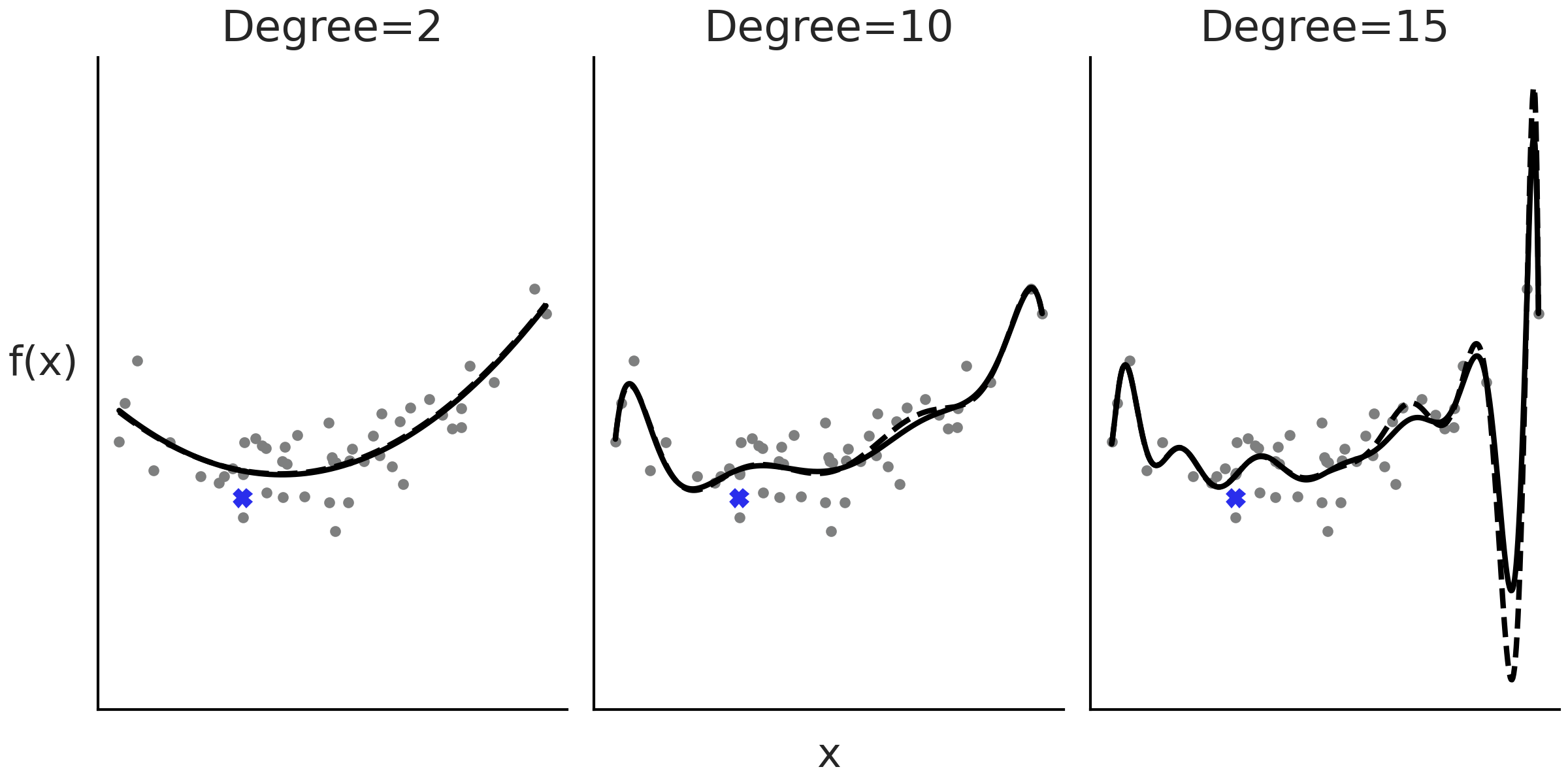
Fig. 5.1 An example of polynomial regression with degrees 2, 10 and 15. As the degree increases the fit gets more wiggly. The dashed lines are the fit when removing the observation indicated with a blue cross. The removal of a data point has a small effect when the degree of polynomial is 2 or 10, but larger when the degree is 15. The fit was calculated using the least squares method.#
One problem with polynomials is that they act globally, when we apply a polynomial of degree \(m\) we are saying that the relationship between the independent and dependent variables is of degree \(m\) for the entire dataset. This can be problematic when different regions of our data need different levels of flexibility. This could lead, for example, to curves that are too flexible [1]. For example, in the last panel of Fig. 5.1 (degree=15), we can see that the fitted curve presents a deep valley followed by a high peak towards high values of \(X\), even when there are no data points with such low or high values.
Additionally, as the degree increases the fit becomes more sensitive to the removal of points, or equivalently to the addition of future data. In other words as the degree increases, the model becomes more prone to overfitting. For example, in Fig. 5.1 the black lines represent the fit to the entire data and the dashed lines the fit when we remove one data point, indicated with a cross in the figure. We can see, especially in the last panel, that removing even a single data point changes the model fit with effects even far away from the location of the point.
5.2. Expanding the Feature Space#
At a conceptual level we can think of polynomial regression as a recipe for creating new predictors, or in more formal terms to expanding the feature space. By performing this expansion we are able to fit a line in the expanded space which gives us a curve on the space of the original data, pretty neat! Nevertheless, feature expansion is not an invitation to statistical anarchy, we can not just apply random transformations to our data and then expect to always get good results. In fact, as we just saw applying polynomials is not problem-free.
To generalize the idea of feature expansion, beyond polynomials we can expand Equation (5.1) into the following form:
where the \(B_i\) are arbitrary functions. In this context we call these functions basis functions. A linear combination of them gives us a function \(f\) that is what we actually “see” as the fit of the model to the data. In this sense the \(B_i\) are an under the hood trick to build a flexible function \(f\).
There are many choices for the \(B_i\) basis functions, we can use polynomials and thus obtain polynomial regression as we just saw, or maybe apply an arbitrary set of functions such as a power of two, a logarithm, or a square root. Such functions may be motivated by the problem at hand, for example, in Section Transforming Covariates we modeled how the length of babies changes with their age by computing the square root of the length, motivated by the fact that human babies, same as other mammals, grow more rapidly in the earlier stages of their life and then the growth tends to level off (similar to how a square root function does).
Another alternative is to use indicator functions like \(I(c_i \leq x_k < c_j)\) to break up the original \(\boldsymbol{X}\) predictor into (non-overlapping) subsets. And then fit polynomial locally, i.e., only inside these subsets. This procedure leads to fitting piecewise polynomials [2] as shown in Fig. 5.2.
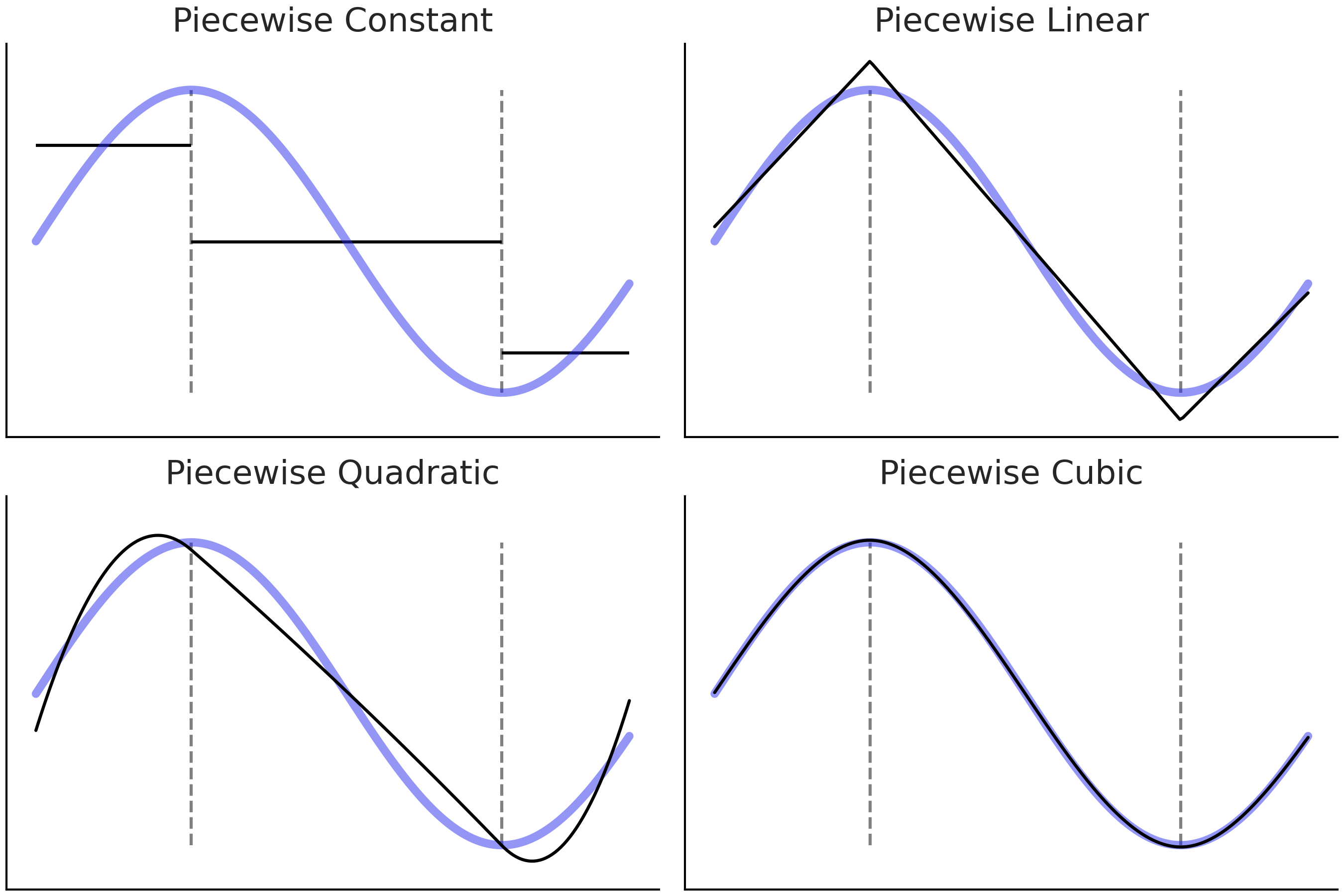
Fig. 5.2 The blue line is the true function we are trying to approximate. The black-solid lines are piecewise polynomials of increasing order (1, 2, 3, and 4). The dashed vertical gray lines are marking the limits of each subdomain on the x-axis.#
In the four panels in Fig. 5.2 the goal is the same, to approximate the blue function. We proceed by first splitting the function into 3 subdomains, delimited by the gray dashed lines, and then we fit a different function to each subdomain. In the first subpanel (piecewise constant) we fit a constant function. We can think of a constant function as a zero degree polynomial. The aggregated solution, i.e. the 3 segments in black is known as a step-function. This may seem to be a rather crude approximation but it may be all that we need. For example, step-functions may be OK if we are trying to find out a discontinuous outcome like the expected mean temperature during morning, afternoon, and night. Or when we are OK about getting a non-smooth approximation even if we think the outcome is smooth [3].
In the second panel (piecewise linear) we do the same as in the first but instead of a constant function we use a linear function, which is a first degree polynomial. Notice that the contiguous linear solutions meet at the dashed lines, this is done on purpose. We could justify this restriction as trying to make the solution as smooth as possible [4].
In the third panel (piecewise quadratic) and fourth panel (piecewise cubic) we use quadratic and cubic piecewise polynomials. As we can see by increasing the degree of the piecewise polynomials we get further and further flexible solutions, which brings better fits but also a higher chance of overfitting.
Because the final fit is a function \(f\) constructed from local solutions (the \(B_i\) basis functions) we can more easily accommodate the flexibility of the model to the demands of the data at different regions. In this particular case, we can use a simpler function (polynomial with lower degree) to fit the data at different regions, while providing a good overall model fit to the whole domain of the data.
So far we have assumed we have a single predictor \(X\), but the same idea can be extended to more than one predictor \(X_0, X_1, \cdots, X_p\). And we can even add an inverse link function \(\phi\) [5] models of this form are known as Generalized Additive Models (GAM): [18, 49].
Recapitulating what we learn in this section, the \(B_i\) functions in Equation (5.3) are a clever statistical device that allows us to fit more flexible models. In principle we are free to choose arbitrary \(B_i\) functions, and we may do it based on our domain knowledge, as a result of an exploratory data analysis phase, or even by trial and error. As not all transformations will have the same statistical properties, it would be nice to have access to some default functions with good general properties over a wider range of datasets. Starting in the next section and for the remainder of this chapter we will restrict the discussion to a family of basis functions known as B-splines [6].
5.3. Introducing Splines#
Splines can be seen as an attempt to use the flexibility of polynomials but keeping them under control and thus obtaining a model with overall good statistical properties. To define a spline we need to define knots [7]. The purpose of the knots is to split the domain of the variable \(\boldsymbol{X}\) into contiguous intervals. For example, the dashed vertical gray lines in Fig. 5.2 represent knots. For our purposes a spline is a piecewise polynomial constrained to be continuous, that is we enforce two contiguous sub-polynomials to meet at the knots. If the sub-polynomials are of degree \(n\) we say the spline is of degree \(n\). Sometimes splines are referred to by their order which would be \(n+1\).
In Fig. 5.2 we can see that as we increase the order of the piecewise polynomial the smoothness of the resulting function also increases. As we already mentioned the sub-polynomials should meet at the knots. On the first panel it may seem we are cheating as there is a step, also known as a discontinuity, between each line, but this is the best we can do if we use constant values at each interval.
When talking about splines, the sub-polynomials are formally known as basis splines or B-splines for short. Any spline function of a given degree can be constructed as a linear combination of basis splines of that degree. Fig. 5.3 shows examples of B-splines of increasing degree from 0 to 3 (top to bottom), the dots at the bottom represent the knots, the blue ones mark the interval at which the highlighted B-spline (in black continuous line) is not zero. All other B-splines are represented with a thinner dashed line for clarity, but all B-splines are equally important. In fact, each subplots in Fig. 5.3 is showing all the B-splines as defined by the given knots. In other words B-splines are completely defined by a set of knots and a degree.
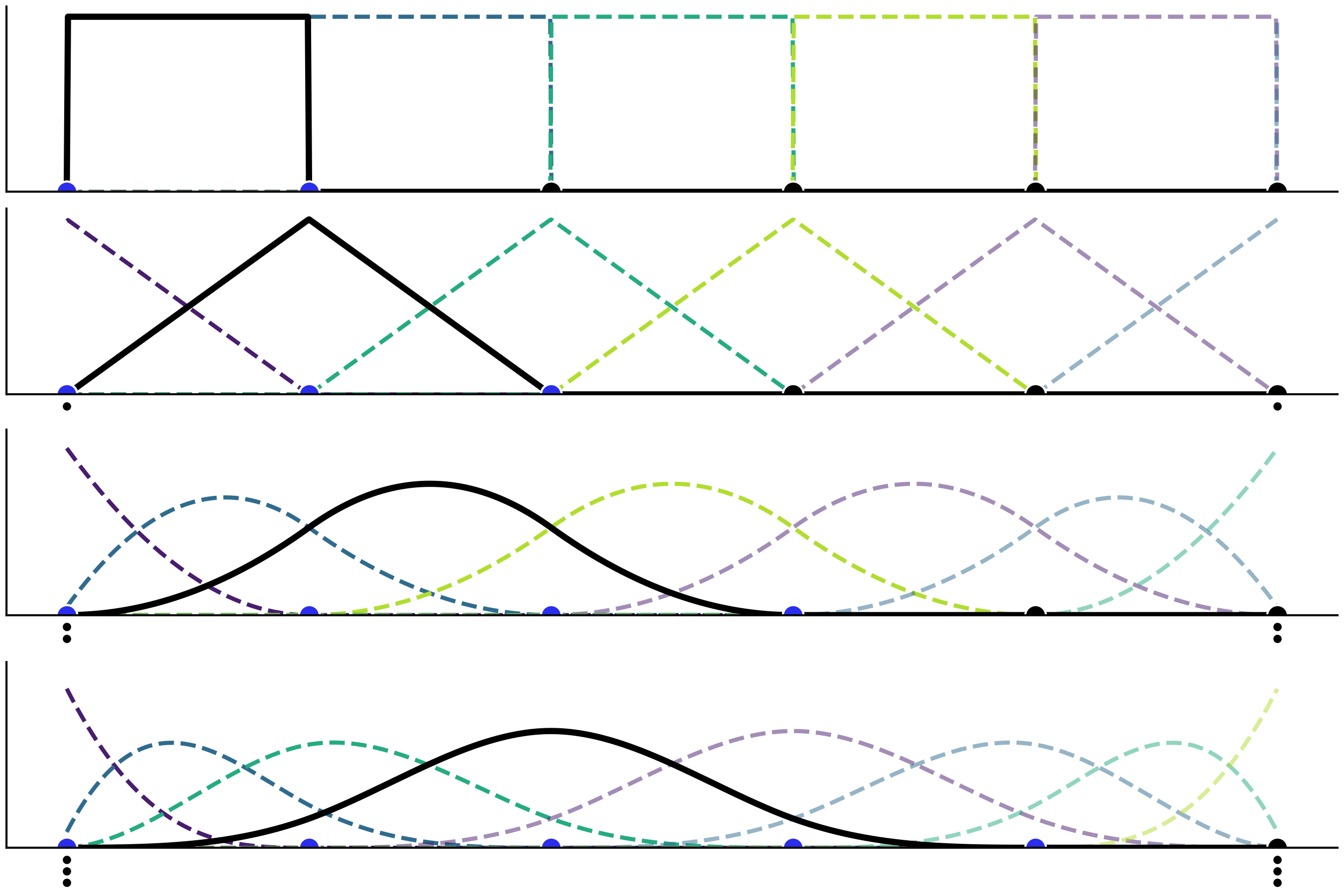
Fig. 5.3 B-splines of increasing degree, from 0 to 3. On the top subplot we have a step function, on second a triangular function and then increasingly Gaussian-like functions. The stacked knots at the boundary (smaller black dots) are added in order to be able to define the splines close to the borders.#
From Fig. 5.3 we can see that as we increase the degree of the B-spline, the domain of the B-spline spans more and more [8]. Thus, for higher degree spline to make sense we need to define more knots. Note that in all cases B-splines are restricted to be non-zero only inside a given interval. This property make splines regression more local than what we would get from a polynomial regression.
As the number of knots controlling each B-splines grows with the degree, for all degrees larger than 0, we are not able to define a B-spline near to the boundaries. This is the reason the B-spline is highlighted in black in Fig. 5.3 to the right as we increase the degree. This presents a potential problem, because it leaves us with less B-splines at the boundaries, so our approximation will suffer there. Fortunately, this boundary problem is easy to solve, we just need to add knots at the boundaries (see the small dots in Fig. 5.3). So if our knots are (0,1,2,3,4,5) and we want to fit a cubic spline (like in the last subplot of Fig. 5.3) we will need to actually use the set of knots (0,0,0,0,1,2,3,4,5,5,5,5). That is, we pad the 0 three times at the beginning and we pad the 5 three times at the end. By doing so we now have the five necessary knots (0,0,0,0,1) to define the first B-spline (see the dashed indigo line that looks like an Exponential distribution in the last subpanel of Fig. 5.3). Then we will use the knots 0,0,0,1,2 to define the second B-spline (the one that looks like a Beta distribution), etc. See how the first complete B-splines (highlighted in black) is defined by the knots (0,1,2,3,4) which are the knots in blue. Notice that we need to pad the knots at the boundaries as many times as the degree of the spline. That is why we have no extra knots for degree 0 and 6 extra knots for degree 3.
Each single B-spline is not very useful on its own, but a linear combination of all of them allows us to fit complex functions. Thus, in practice fitting splines requires that we choose the order of the B-splines, the number and locations of knots and then find the set of coefficients to weight each B-spline. This is represented in Fig. 5.4. We can see the basis functions represented using a different color to help individualize each individual basis function. The knots are represented with black dots at the bottom of each subplot. The second row is more interesting as we can see the same basis functions from the first row scaled by a set of \(\beta_i\) coefficients. The thicker continuous black line represents the spline that is obtained by a weighted sum of the B-splines with the weights given by the \(\beta\) coefficients.
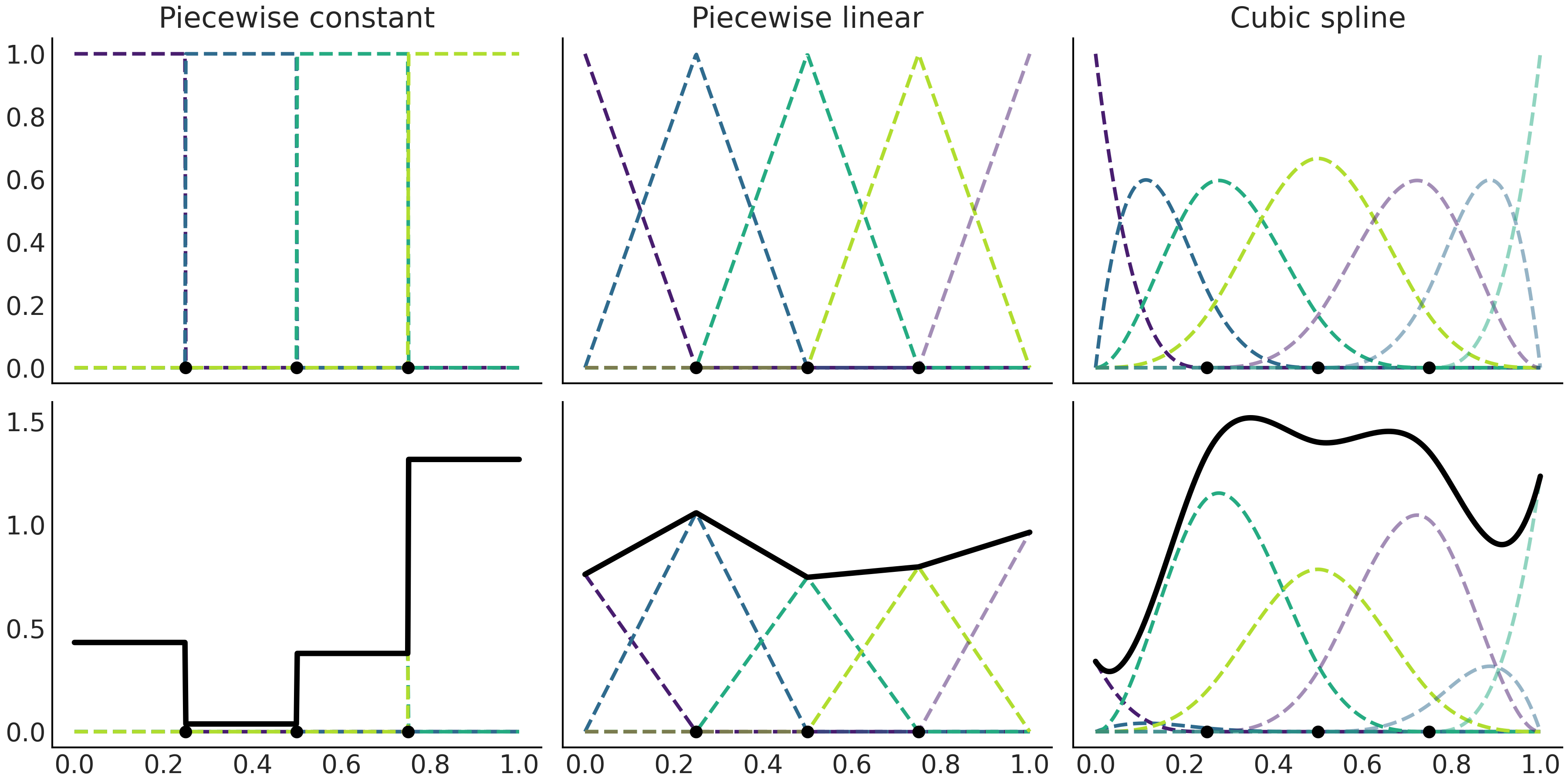
Fig. 5.4 B-splines defined using Patsy. On the first row we can see splines of increasing order 1 (piecewise constant), 2 (piecewise linear) and 4 (cubic) represented with gray dashed lines. For clarity each basis function is represented with a different color. On the second row we have the basis splines from the first row scaled by a set of coefficients. The thick black line represents the sum of these basis functions. Because the value of the coefficients was randomly chosen we can see each sub-panel in the second row as a random sample from a prior distribution over the spline space.#
In this example we generated the \(\beta_i\) coefficients by sampling from a Half Normal distribution (Line 17 in Code Block splines_patsy_plot). Thus, each panel in Fig. 5.4 is showing only one realization of a probability distribution over splines. You can easily see this is true by removing the random seed and running Code Block splines_patsy_plot a few times, each time you will see a different spline. Additionally, you may also try replacing the Half Normal distribution, with another one like the Normal, Exponential, etc. Fig. 5.5 shows four realization of cubic splines.
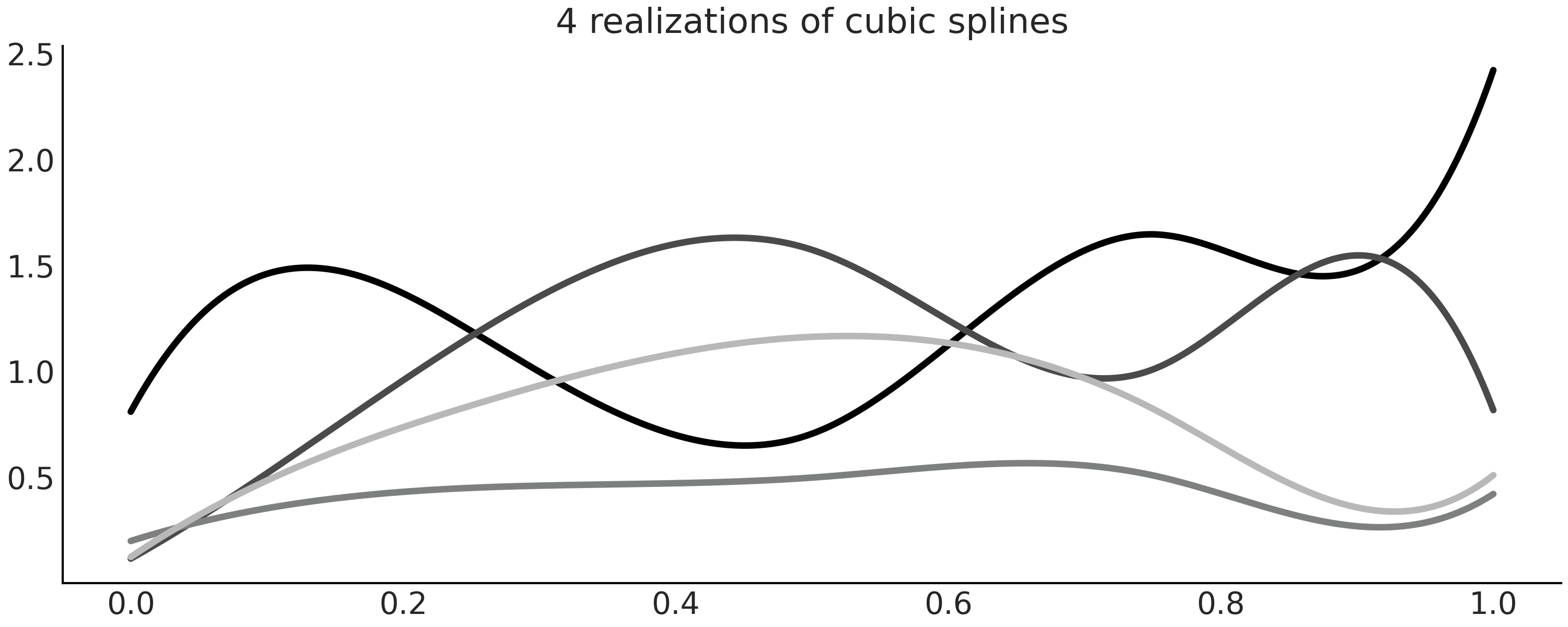
Fig. 5.5 Four realizations of cubic splines with \(\beta_i\) coefficients sampled from a Half Normal distribution.#
Four is a crowd for splines
Of all possible splines, probably cubic splines are the most commonly used. But why are cubic splines the queen of splines? Figures Fig. 5.2 and Fig. 5.4 offer some hints. Cubic splines provide us with the lowest order of splines able to generate smooth enough curves for most common scenarios, rendering higher order splines less attractive. What do we mean by smooth enough? Without going into the mathematical details, we meant that the fitted function does not present sudden changes of slope. One way of doing this is by adding the restriction that two contiguous piecewise polynomials should meet at their common knots. Cubic splines have two additional restrictions, the first and second derivatives are also continuous, meaning that the slope is continuous at the knots and also the slope of the slope [9]. In fact, a spline of degree \(m\) will have \(m-1\) derivatives at the knots. Having said all that, splines of lower or higher order can still be useful for some problems, it is just that cubic splines are good defaults.
5.4. Building the Design Matrix using Patsy#
In Figures Fig. 5.3 and
Fig. 5.4 we plot the B-splines, but so far we have
omitted how to compute them. The main reason is that computation can be
cumbersome and there are already efficient algorithms available in
packages like Scipy [10]. Thus, instead of discussing how the B-splines
can be computed from scratch we are going to rely on Patsy, a package
for describing statistical models, especially linear models, or models
that have a linear component, and building design matrices. It is
closely inspired by the formula mini-language widely used in many
packages from the R programming language ecosystem. Just for you to get
a taste of the formula language, a linear model with two covariates
looks like "y ~ x1 + x2" and if we want to add an interaction we can
write "y ~ x1 + x2 + x1:x2". This is a similar syntax as the one shown
in Chapter 3 in the box highlighting Bambi. For more
details please check the patsy documentation [11].
To define a basis spline design matrix in Patsy we need to pass a string
to the dmatrix function starting with the particle bs(), while
this particle is a string is parsed by Patsy as a function. And thus it
can also take several arguments including the data, an array-like of
knots indicating their location and the degree of the spline. In Code
Block splines_patsy we define 3 design
matrices, one with degree 0 (piecewise constant), another with degree 1
(piecewise linear) and finally one with degree 3 (cubic spline).
x = np.linspace(0., 1., 500)
knots = [0.25, 0.5, 0.75]

B0 = dmatrix("bs(x, knots=knots, degree=0, include_intercept=True) - 1",
             {"x": x, "knots":knots})
B1 = dmatrix("bs(x, knots=knots, degree=1, include_intercept=True) - 1",
             {"x": x, "knots":knots})
B3 = dmatrix("bs(x, knots=knots, degree=3,include_intercept=True) - 1",
             {"x": x, "knots":knots})
Fig. 5.6 represents the 3 design matrices computed
with Code Block splines_patsy. To better
grasp what Patsy is doing we also recommend you use Jupyter notebook/lab
or your favorite IDE to inspect the objects B0, B1 and B2.
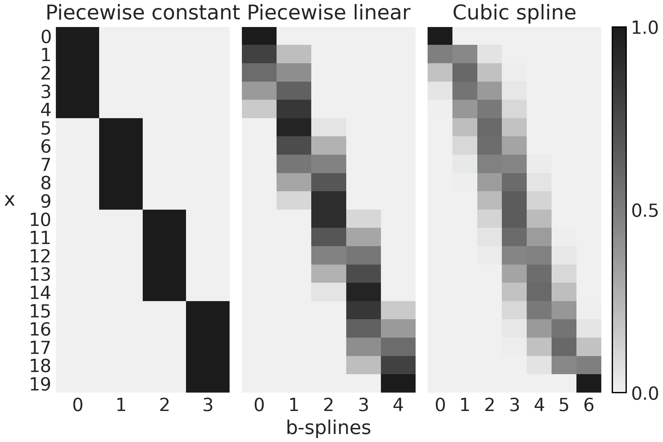
Fig. 5.6 Design matrices generated with Patsy in Code Block splines_patsy. The color goes from black (1) to light-gray (0), the number of columns is the number of B-splines and the number of rows the number of datapoints.#
The first subplot of Fig. 5.6 corresponds to B0,
a spline of degree 0. We can see that the design matrix is a matrix with
only zeros (light-gray) and ones (black). The first B-spline (column 0)
is 1 for the first 5 observations and 0 otherwise, the second B-spline
(column 1) is 0 for the first 5 observations, 1 for the second 5
observations and 0 again. And the same pattern is repeated. Compare this
with the first subplot (first row) of Fig. 5.4,
you should see how the design matrix is encoding that plot.
For the second subplot in Fig. 5.6 we have the first B-spline going from 1 to 0, the second, third and fourth goes from 0 to 1 and then back from 1 to 0. The fifth B-spline goes from 0 to 1. You should see how this patterns match the line with negative slope, the 3 triangular functions and the line with positive slope in the second subplot (first row) of Fig. 5.4.
Finally we can see something similar if we compare how the 7 columns in the third subplot in Fig. 5.6 match the 7 curves in the third subplot (first row) of Fig. 5.4.
Code Block splines_patsy was used to
generate the B-splines in Figures Fig. 5.4 and
Fig. 5.6, the only different is that for the former
we used x = np.linspace(0., 1., 500), so the curves look smoother and
we use x = np.linspace(0., 1., 20) in the later so the matrices are
easier to understand.
_, axes = plt.subplots(2, 3, sharex=True, sharey="row")
for idx, (B, title) in enumerate(zip((B0, B1, B3),
                                     ("Piecewise constant",
                                      "Piecewise linear",
                                      "Cubic spline"))):
    # plot spline basis functions
    for i in range(B.shape[1]):
        axes[0, idx].plot(x, B[:, i],
                          color=viridish[i], lw=2, ls="--")
    # we generate some positive random coefficients
    # there is nothing wrong with negative values
    β = np.abs(np.random.normal(0, 1, size=B.shape[1]))
    # plot spline basis functions scaled by its β
    for i in range(B.shape[1]):
        axes[1, idx].plot(x, B[:, i]*β[i],
                          color=viridish[i], lw=2, ls="--")
    # plot the sum of the basis functions
    axes[1, idx].plot(x, np.dot(B, β), color="k", lw=3)
    # plot the knots
    axes[0, idx].plot(knots, np.zeros_like(knots), "ko")
    axes[1, idx].plot(knots, np.zeros_like(knots), "ko")
    axes[0, idx].set_title(title)
So far we have explored a couple of examples to gain intuition into what splines are and how to automate their creation with the help of Patsy. We can now move forward into computing the weights. Let us see how we can do that in a Bayesian model with PyMC3.
5.5. Fitting Splines in PyMC3#
In this section we are going to use PyMC3 to obtain the values of the regression coefficients \(\beta\) by fitting a set of B-splines to the data.
Modern bike sharing systems allow people in many cities around the globe to rent and return bikes in a completely automated fashion, helping to increase the efficiency of the public transportation and probably making part of the society healthier and even happier. We are going to use a dataset from such a bike sharing system from the University of California Irvine’s Machine Learning Repository [12]. For our example we are going to estimate the number of rental bikes rented per hour over a 24 hour period. Let us load and plot the data:
data = pd.read_csv("../data/bikes_hour.csv")
data.sort_values(by="hour", inplace=True)

# We standardize the response variable
data_cnt_om = data["count"].mean()
data_cnt_os = data["count"].std()
data["count_normalized"] = (data["count"] - data_cnt_om) / data_cnt_os
# Remove data, you may later try to refit the model to the whole data
data = data[::50]
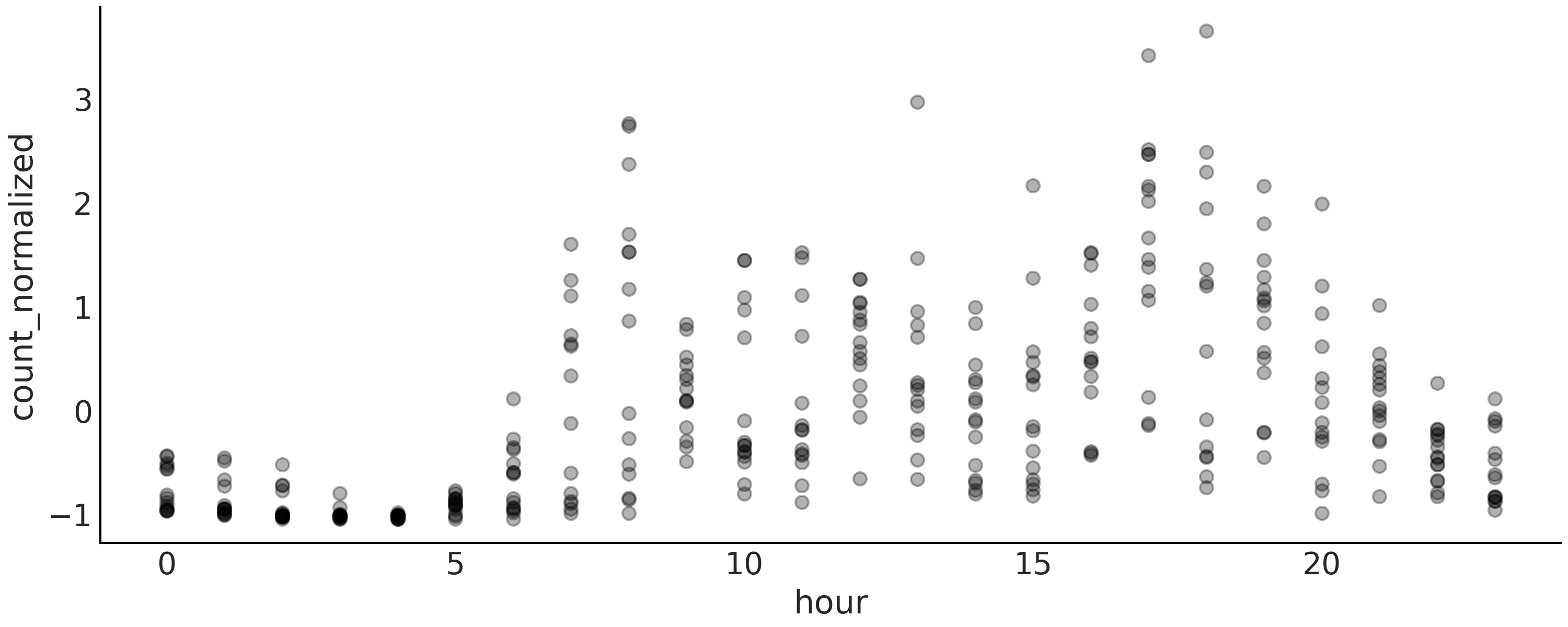
Fig. 5.7 A visualization of the bikes data. Each point is the normalized number of bikes rented per hour of the day (on the interval 0, 23). The points are semi-transparent to avoid excessive overlapping of points and thus help see the distribution of the data.#
A quick look at Fig. 5.7 shows that the relationship between the hour of the day and the number of rental bikes is not going to be very well captured by fitting a single line. So, let us try to use a spline regression to better approximate the non-linear pattern.
As we already mentioned in order to work with splines we need to define the number and position of the knots. We are going to use 6 knots and use the simplest option to position them, equal spacing between each knot.
num_knots = 6
knot_list = np.linspace(0, 23, num_knots+2)[1:-1]
Notice that in Code Block knot_list we define 8 knots, but then we remove the first and last knots, ensuring we keep 6 knots which are defined in the interior of the data. Whether this is a useful strategy will depends on the data. For example, if the bulk of the data is away from the borders this will be a good idea, also the larger the number of knots the less important their positions.
Now we use Patsy to define and build the design matrix for us
B = dmatrix(
    "bs(cnt, knots=knots, degree=3, include_intercept=True) - 1",
    {"cnt": data.hour.values, "knots": knot_list[1:-1]})
The proposed statistical model is:
Our spline regression model is very similar to the linear models from Chapter 3. All the hard-work is done by the design matrix \(\boldsymbol{B}\) and its expansion of the feature space. Notice that we are using linear algebra notation to write the multiplications and sums of Equations (5.3) and (5.4) in a shorter form, that is we write \(\boldsymbol{\mu} = \boldsymbol{B}\boldsymbol{\beta}\) instead of \(\boldsymbol{\mu} = \sum_i^n B_i \boldsymbol{\beta}_i\).
As usual the statistical syntax is translated into PyMC3 in nearly a one-to-one fashion.
with pm.Model() as splines:
    τ = pm.HalfCauchy("τ", 1)
    β = pm.Normal("β", mu=0, sd=τ, shape=B.shape[1])
    μ = pm.Deterministic("μ", pm.math.dot(B, β))
    σ = pm.HalfNormal("σ", 1)
    c = pm.Normal("c", μ, σ, observed=data["count_normalized"].values)
    idata_s = pm.sample(1000, return_inferencedata=True)
We show in Fig. 5.8 the final fitted linear prediction as a solid black line and each weighted B-spline as a dashed line. It is a nice representation as we can see how the B-splines are contributing to the final result.
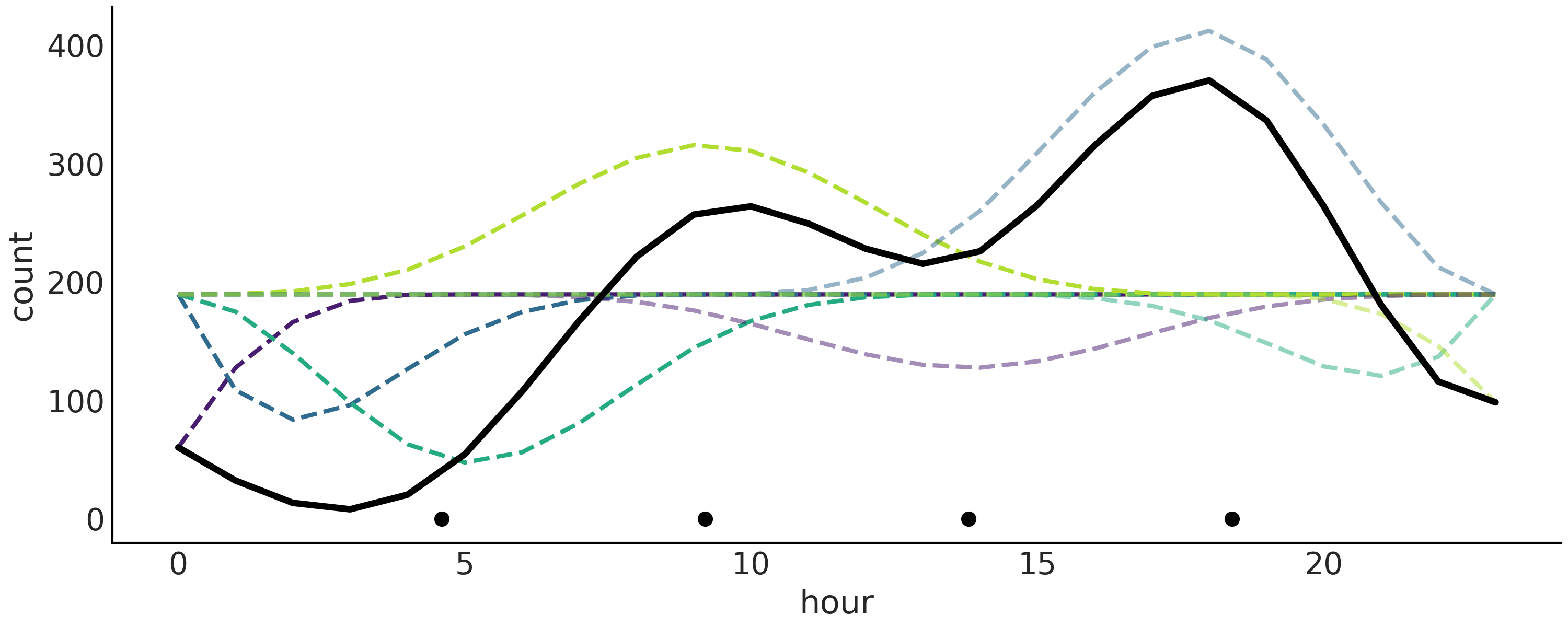
Fig. 5.8 Bikes data fitted using splines. The B-splines are represented with dashed lines. The sum of them generates the thicker solid black line. The plotted values correspond to mean values from the posterior. The black dots represent the knots. The splines in this figure look very jagged, relative to the splines plotted in Fig. 5.4. The reason is that we are evaluating the function in fewer points. 24 points here because the data is binned per hour compared to 500 in Fig. 5.4.#
A more useful plot when we want to display the results of the model is to plot the data with the overlaid splines and its uncertainty as in Fig. 5.9. From this figure we can easily see that the number of rental bikes is at the lowest number late at night. There is then an increase, probably as people wake up and go to work. We have a first peak at around hour 10, which levels-off, or perhaps slightly declines, then followed by a second peak as people commute back home at around hour 18, after which there a steady decline.
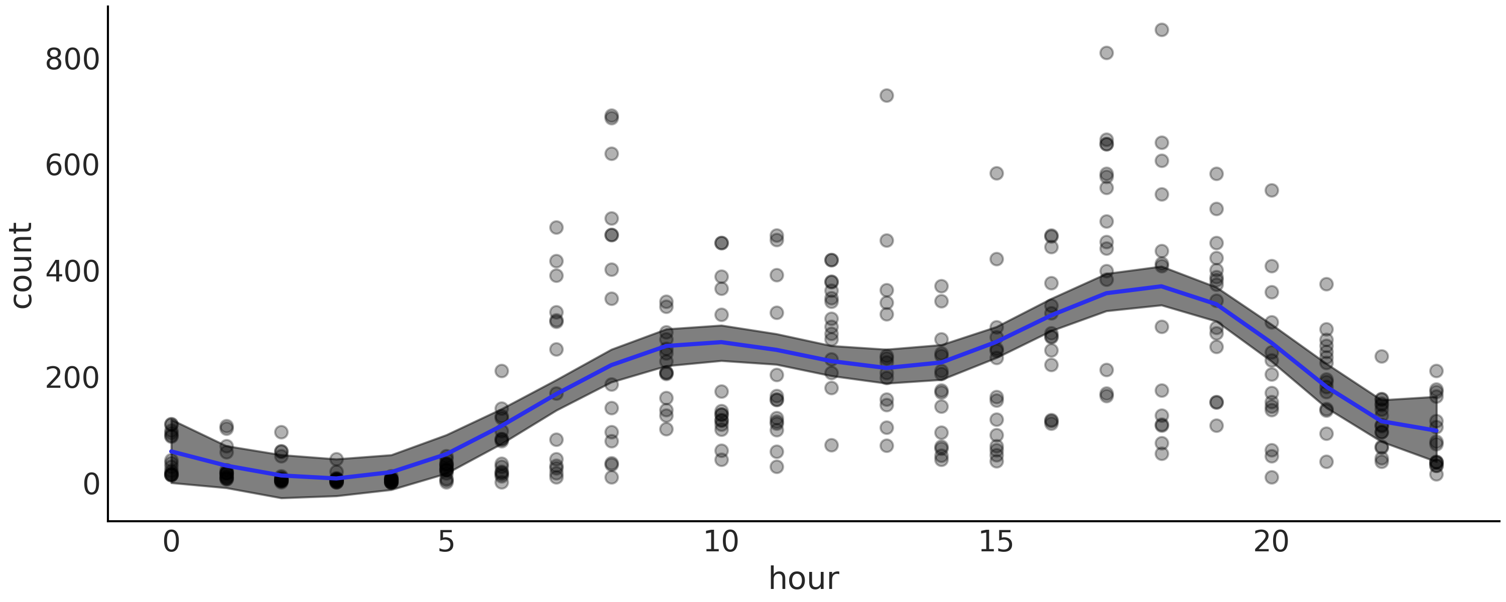
Fig. 5.9 Bikes data (black dots) fitted using splines. The shaded curve represents the 94% HDI interval (of the mean) and the blue curve represents the mean trend.#
In this bike rental example we are dealing with a circular variable,
meaning that hour 0 is equal to the hour 24. This may be more or less
obvious to us, but it is definitely not obvious to our model. Patsy
offers a simple solution to tell our model that the variable is
circular. Instead of defining the design matrix using bs we can use
cc, this is a cubic spline that is circular-aware. We recommend you
check the Patsy documentation for more details and explore using cc in
the previous model and compare results.
5.6. Choosing Knots and Prior for Splines#
One modeling decision we have to make when working with splines is to choose the number and location of the knots. This can be a little bit concerning, given that in general the number of knots and their spacing are not obvious decisions. When faced with this type of choice we can always try to fit more than one model and then use methods such as LOO to help us pick the best model. Table 5.1 shows the results of fitting a model like the one defined in Code Block splines with, 3, 6, 9, 12, and 18 equally distanced knots. We can see that the spline with 12 knots is selected by LOO as the best model.
One interesting observation from Table 5.1, is that
the weights are 0.88 for model m_12k (the top ranked model) and 0.12
to m_3k (the last ranked model). With virtually 0 weight for the rest
of the models. As we explained in Section Model Averaging
by default the weights are computed using stacking, which is a method
that attempts to combine several models in a meta-model in order to
minimize the divergence between the meta-model and the true generating
model. As a result even when models m_6k, m_9k and m_18k have
better values of loo, once m_12k is included they do not have much
to add and while m_3k is the lowest ranked model, it seems that it
still has something new to contribute to the model averaging.
Fig. 5.10 show the mean fitted spline for all
these models.
rank |
loo |
p_loo |
d_loo |
weight |
se |
dse |
warning |
loo_scale |
|
m_12k |
0 |
-377.67 |
14.21 |
0.00 |
0.88 |
17.86 |
0.00 |
False |
log |
m_18k |
1 |
-379.78 |
17.56 |
2.10 |
0.00 |
17.89 |
1.45 |
False |
log |
m_9k |
2 |
-380.42 |
11.43 |
2.75 |
0.00 |
18.12 |
2.97 |
False |
log |
m_6k |
3 |
-389.43 |
9.41 |
11.76 |
0.00 |
18.16 |
5.72 |
False |
log |
m_3k |
4 |
-400.25 |
7.17 |
22.58 |
0.12 |
18.01 |
7.78 |
False |
log |
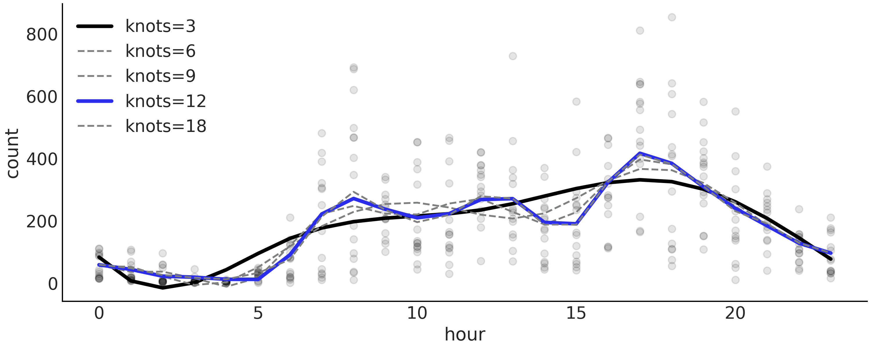
Fig. 5.10 Mean posterior spline for the model described in Code Block
splines with different number of knots (3, 6,
9, 12, 18) . Model m_12k is highlighted in blue as the top ranked
model according to LOO. Model m_3k is highlighted in black, while the
rest of the models are in grayed-out as they have being assigned a
weight of zero (see Table 5.1).#
One piece of advice that may help decide the locations of knots is to
place them based on quantiles, instead of uniformly. In Code Block
knot_list we could have defined the
knot_list using
knot_list = np.quantile(data.hour, np.linspace(0, 1, num_knots)). In
this way we will be putting more knots where we have more data and less
knots where less data. This translates into a more flexible
approximation for data-richer portions.
5.6.1. Regularizing Prior for Splines#
As choosing too few knots could lead to under-fitting and too many to overfitting, we may want to use a rather large number of knots and then choose a regularizing prior. From the definition of splines and Fig. 5.4 we can see that the closer the consecutive \(\boldsymbol{\beta}\) coefficients are to each other, the smoother the resulting function will be. Imagine you are dropping two consecutive columns of the design matrix in Fig. 5.4, effectively setting those coefficients to 0, the fit will be much less smooth as we do not have enough information in the predictor to cover some sub region (recall that splines are local). Thus we can achieve smoother fitted regression line by choosing a prior for the \(\boldsymbol{\beta}\) coefficients in such a way that the value of \(\beta_{i+1}\) is correlated with the value of \(\beta_{i}\):
Using PyMC3 we can write an equivalent version using a Gaussian Random Walk prior distribution:
To see the effect of this prior we are going to repeat the analysis of
the bike dataset, but this time using num_knots = 12. We refit the
data using splines model and the following model:
with pm.Model() as splines_rw:
    τ = pm.HalfCauchy("τ", 1)
    β = pm.GaussianRandomWalk("β", mu=0, sigma=τ, shape=B.shape[1])
    μ = pm.Deterministic("μ", pm.math.dot(B, β))
    σ = pm.HalfNormal("σ", 1)
    c = pm.Normal("c", μ, σ, observed=data["count_normalized"].values)
    trace_splines_rw = pm.sample(1000)
On Fig. 5.11 we can see that the spline mean
function for the model splines_rw (black line) is less wiggly than the
spline mean function without smoothing prior (gray thick line), although
we admit that the difference seems to be rather small.
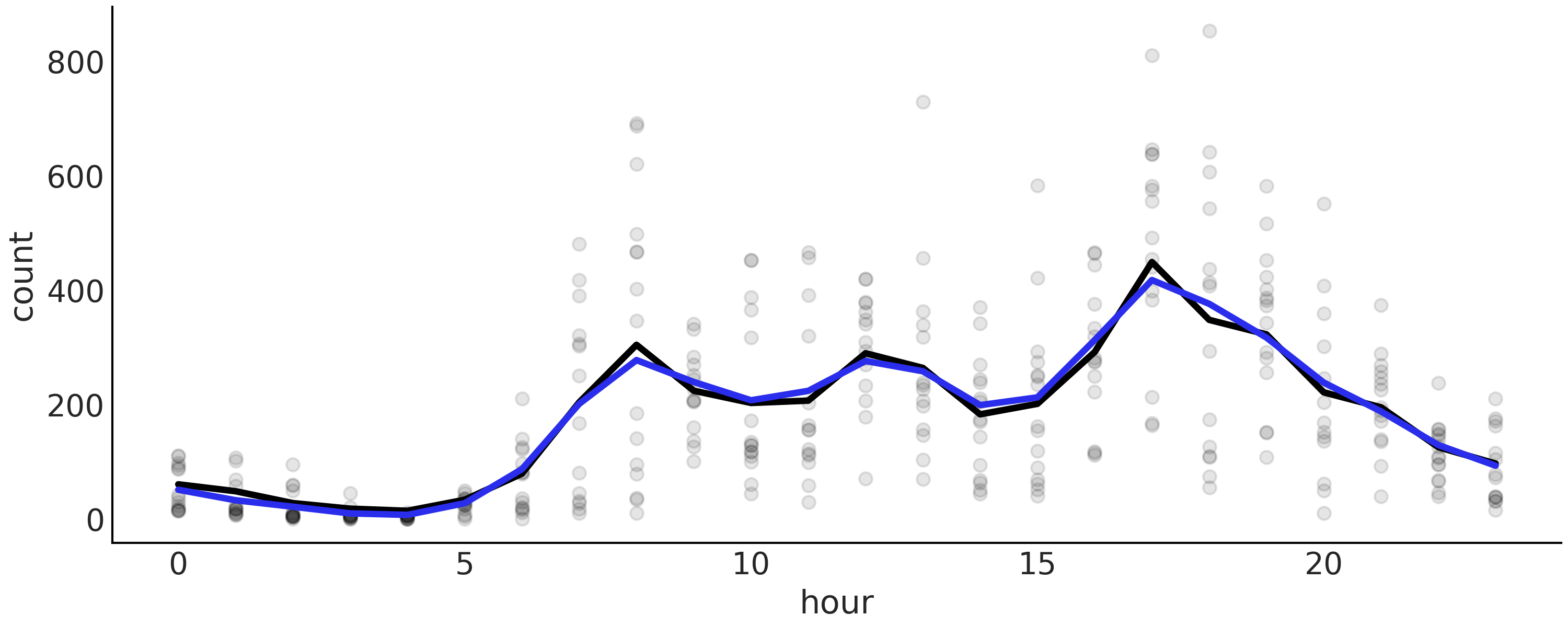
Fig. 5.11 Bikes data fitted with either a Gaussian prior (black) or a regularizing
Gaussian Random Walk Prior (blue). We use 22 knots for both cases. The
black line corresponds to the mean spline function computed from
splines model. The blue line is the mean function for the model
splines_rw.#
5.7. Modeling CO₂ Uptake with Splines#
For a final example of splines we are going to use data from an experimental study [50, 51]. The experiment consists of measuring the CO₂ uptake in 12 different plants under varying conditions. Here we will only explore the effect of the external CO₂ concentration, i.e. how the CO₂ concentration in the environment affects the consumption of CO₂ by different plants. The CO₂ uptake was measured at seven CO₂ concentrations for each plant, the same seven values for each one of the 12 plants. Let us begin by loading and tidying up the data.
plants_CO2 = pd.read_csv("../data/CO2_uptake.csv")
plant_names = plants_CO2.Plant.unique()

# Index the first 7 CO2 measurements per plant
CO2_conc = plants_CO2.conc.values[:7]

# Get full array which are the 7 measurements above repeated 12 times
CO2_concs = plants_CO2.conc.values
uptake = plants_CO2.uptake.values

index = range(12)
groups = len(index)
The first model we are going to fit is one with a single response curve,
i.e. assuming the response curve is the same for all the 12 plants. We
first define the design matrix, using Patsy, just as we previously did.
We set num_knots=2 because we have 7 observations per plant, so a
relatively low number of knots should work fine. In Code Block
plants_co2_import, CO2_concs is a
list with the values [95, 175, 250, 350, 500, 675, 1000] repeated 12
times, one time per plant.
num_knots = 2
knot_list = np.linspace(CO2_conc[0], CO2_conc[-1], num_knots+2)[1:-1]

Bg = dmatrix(
    "bs(conc, knots=knots, degree=3, include_intercept=True) - 1",
    {"conc": CO2_concs, "knots": knot_list})
This problem looks similar to the bike rental problem from previous sections and thus we can start by applying the same model. Using a model that we have already applied in some previous problem or the ones we learned from the literature is a good way to start an analysis. This model-template approach can be viewed as a shortcut to the otherwise longer process of model design [17]. In addition to the obvious advantage of not having to think of a model from scratch, we have other advantages such as having better intuition of how to perform exploratory analysis of the model and then possible routes for making changes into the model either to simplify it or to make it more complex.
with pm.Model() as sp_global:
    τ = pm.HalfCauchy("τ", 1)
    β = pm.Normal("β", mu=0, sigma=τ, shape=Bg.shape[1])
    μg = pm.Deterministic("μg", pm.math.dot(Bg, β))
    σ = pm.HalfNormal("σ", 1)
    up = pm.Normal("up", μg, σ, observed=uptake)
    idata_sp_global = pm.sample(2000, return_inferencedata=True)
From Fig. 5.12 we can clearly see that the model is only providing a good fit for some of the plants. The model is good on average, i.e. if we pool all the species together, but not very good for specific plants.
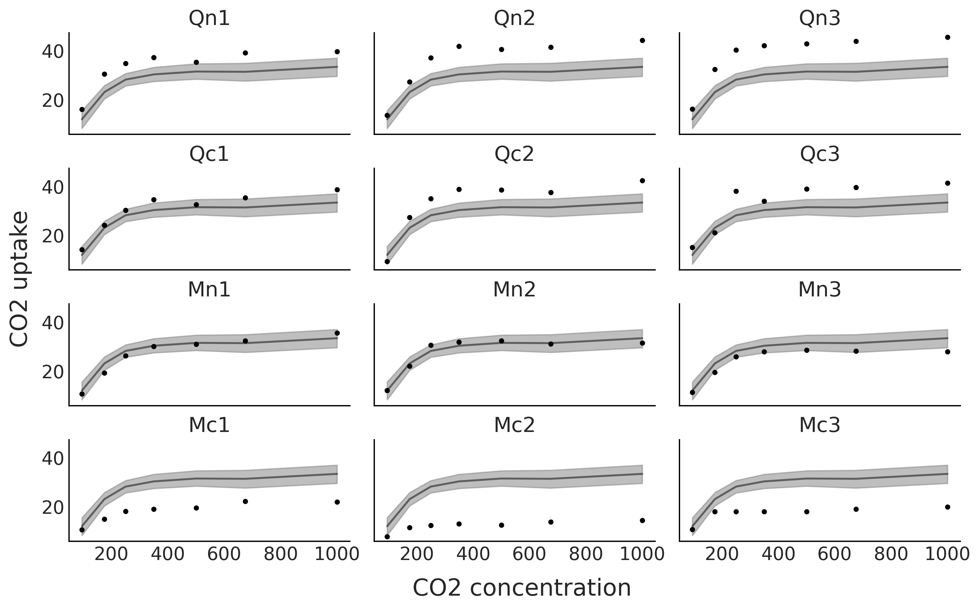
Fig. 5.12 The black dots represents the CO₂ uptake measured at seven CO₂ concentrations for each one of 12 plants (Qn1, Qn2, Qn3, Qc1, Qc2, Qc3, Mn1, Mn2, Mn3, Mc1, Mc2, Mc3). The black line is the mean spline fit from the model in Code Block sp_global and the gray shaded curve represents the 94% HDI interval for that fit.#
Let us try now with a model with a different response per plant, in
order to do this we define the design matrix Bi in Code Block
Bi_matrix. To define Bi we use the list
CO2_conc = [95, 175, 250, 350, 500, 675, 1000], thus Bi is a
\(7 \times 7\) matrix while Bg is a \(84 \times 7\) matrix.
Bi = dmatrix(
    "bs(conc, knots=knots, degree=3, include_intercept=True) - 1",
    {"conc": CO2_conc, "knots": knot_list})
Accordingly with the shape of Bi, the parameter \(\beta\) in Code Block
sp_individual has now shape
shape=(Bi.shape[1], groups)) (instead of shape=(Bg.shape[1]))) and
we reshape μi[:,index].T.ravel()
with pm.Model() as sp_individual:
    τ = pm.HalfCauchy("τ", 1)
    β = pm.Normal("β", mu=0, sigma=τ, shape=(Bi.shape[1], groups))
    μi = pm.Deterministic("μi", pm.math.dot(Bi, β))
    σ = pm.HalfNormal("σ", 1)
    up = pm.Normal("up", μi[:,index].T.ravel(), σ, observed=uptake)
    idata_sp_individual = pm.sample(2000, return_inferencedata=True)
From Fig. 5.13 we can now see that we have a much better fit for each one of the 12 plants.
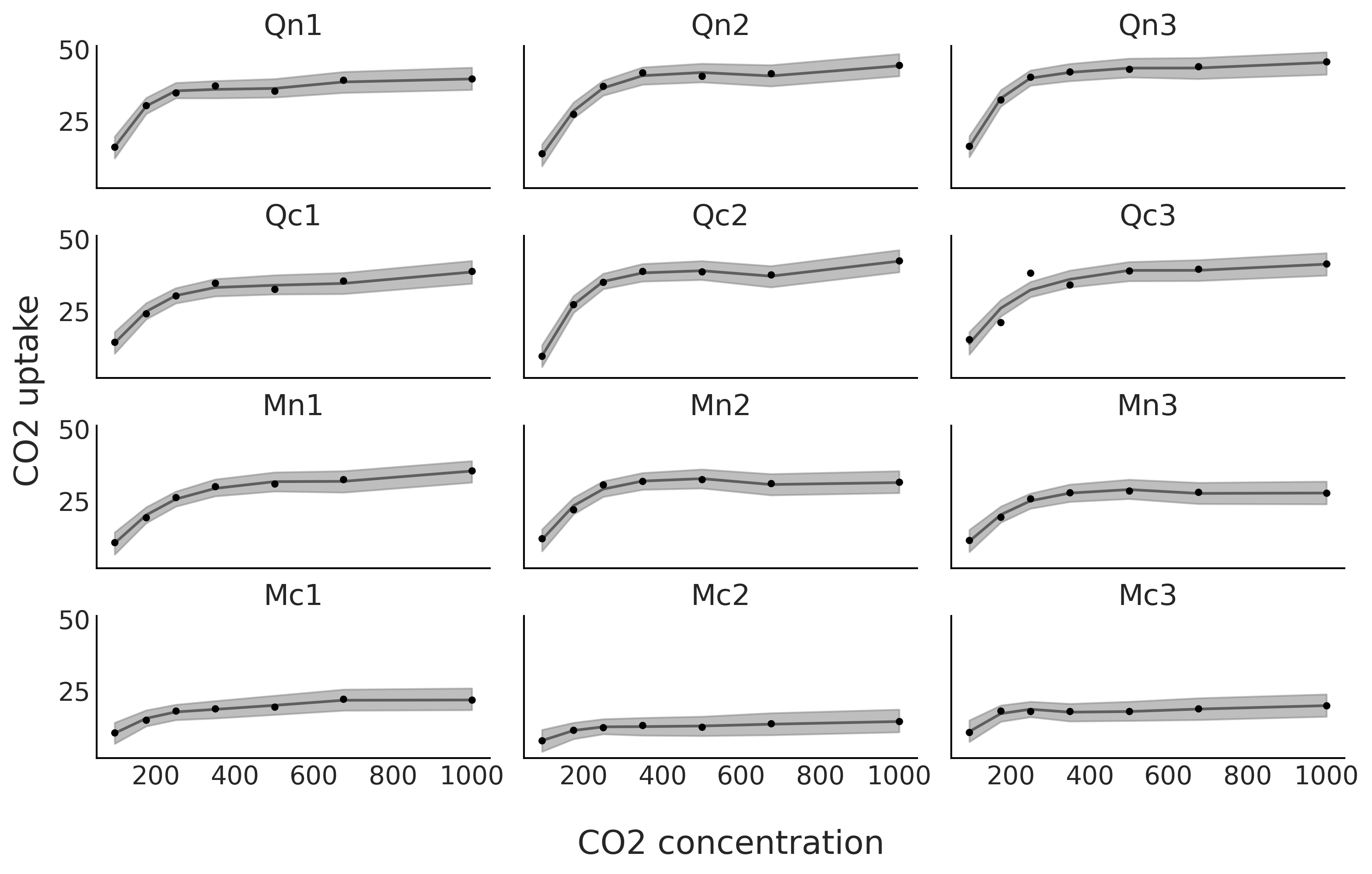
Fig. 5.13 CO₂ uptake measured at seven CO₂ concentrations for 12 plants. The black line is the mean spline fit from the model in Code Block sp_individual and the gray shaded curve represents the 94% HDI interval for that fit.#
We can also mix both previous models [13]. This may be interesting if
we want to estimate a global trend for the 12 plants plus individual
fits. Model sp_mix in Code Block sp_mix use
both previously defined design matrices Bg and Bi.
with pm.Model() as sp_mix:
    τ = pm.HalfCauchy("τ", 1)
    βg = pm.Normal("βg", mu=0, sigma=τ, shape=Bg.shape[1])
    μg = pm.Deterministic("μg", pm.math.dot(Bg, βg))
    βi = pm.Normal("βi", mu=0, sigma=τ, shape=(Bi.shape[1], groups))
    μi = pm.Deterministic("μi", pm.math.dot(Bi, βi))
    σ = pm.HalfNormal("σ", 1)
    up = pm.Normal("up", μg+μi[:,index].T.ravel(), σ, observed=uptake)
    idata_sp_mix = pm.sample(2000, return_inferencedata=True)
Fig. 5.14 show the fit of model sp_mix. One
advantage of this model is that we can decompose the individual fit (in
blue) into two terms, a global trend, in black, and the deviation of
that trend for each plant, in gray. Notice how the global trend, in
black, is repeated in each subplot. We can see that the deviations are
different not only in the average uptake, i.e. they are not flat
straight lines, but they are also different, to various extents, in the
shape of their functional responses.
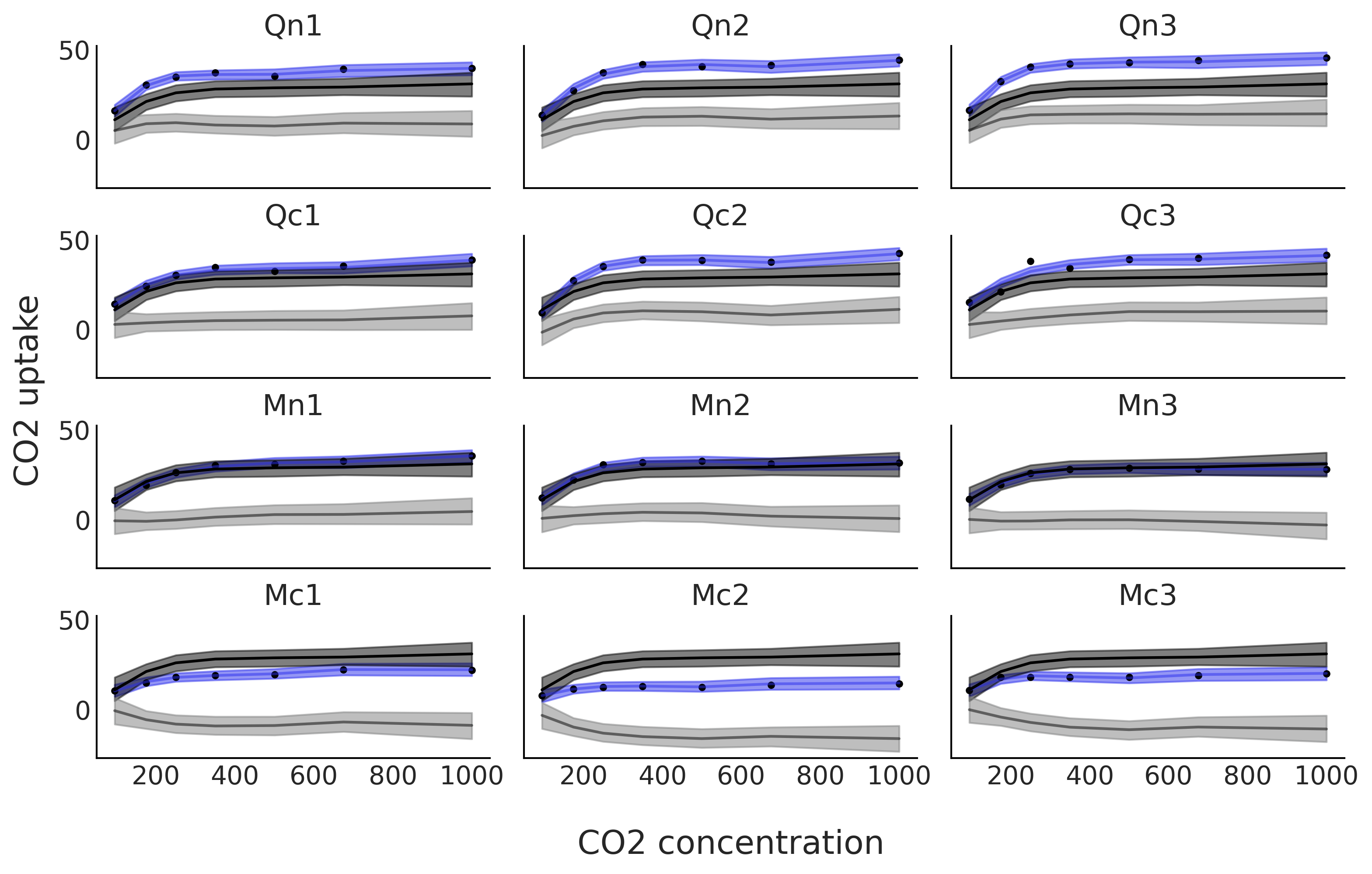
Fig. 5.14 CO₂ uptake measured at seven CO₂ concentrations for 12 plants. The blue line is the mean spline fit from model in Code Block sp_mix and the gray shaded curve represents the 94% HDI interval for that fit. This fit is decomposed into two terms. In black, and a dark gray band, the global contribution and in gray, and a light gray band, the deviations from that global contribution. The blue line, and blue band, is the sum of the global trend and deviations from it.#
Fig. 5.15 shows that according to LOO sp_mix is a
better model than the other two. We can see there is still some
uncertainty about this statement as the standard errors for models
sp_mix and sp_individual partially overlap. We can also see that
models sp_mix and sp_individual are penalized harder than
sp_global (the distance between the empty circle and black circle is
shorter for sp_global). We note that LOO computation returns warnings
about the estimated shape parameter of Pareto distribution being greater
than 0.7. For this example we are going to stop here, but for a real
analysis, we should pay further attention to these warnings and try to
follow some of the actions described in Section Pareto Shape Parameter.
cmp = az.compare({"global":idata_sp_global,
                  "individual":idata_sp_individual,
                  "mix":idata_sp_mix})
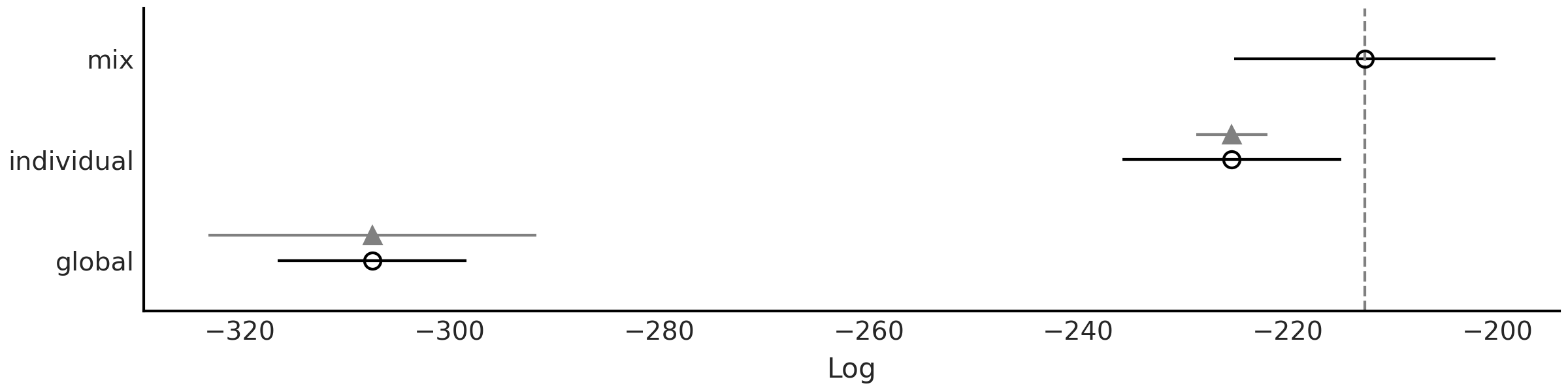
Fig. 5.15 Model comparison using LOO for the 3 different CO₂ uptake models
discussed in this chapter (sp_global, sp_individual, sp_mix).
Models are ranked from higher predictive accuracy to lower. The open
dots represent the values of LOO, the black dots are the in-sample
predictive accuracy. The black segments represent the standard error for
the LOO computations. The gray segments, centered at the triangles,
represent the standard errors of the difference between the values of
LOO for each model and the best ranked model.#
5.8. Exercises#
5E1.. Splines are quite powerful so its good to know when and where to use them. To reinforce this explain each of the following
The differences between linear regression and splines.
When you may want to use linear regression over splines
Why splines is usually preferred over polynomial regression of high order.
5E2. Redo Fig. 5.1 but fitting a polynomial of degree 0 and of degree 1. Does they look similar to any other type of model. Hint: you may want to use the code in the GitHub repository.
5E3. Redo Fig. 5.2 but changing the value of one or the two knots. How the position of the knots affects the fit? You will find the code in the GitHub repository.
5E4. Below we provide some data. To each data fit a 0,
1, and 3 degree spline. Plot the fit, including the data and position of
the knots. Use knots = np.linspace(-0.8, 0.8, 4). Describe the fit.
x = np.linspace(-1, 1., 200)andy = np.random.normal(2*x, 0.25)x = np.linspace(-1, 1., 200)andy = np.random.normal(x**2, 0.25)pick a function you like.
5E5. In Code Block bikes_dmatrix we used a non-cyclic aware design matrix. Plot this design matrix. Then generate a cyclic design matrix. Plot this one too what is the difference?
5E6. Generate the following design matrices using Patsy.
x = np.linspace(0., 1., 20)
knots = [0.25, 0.5, 0.75]

B0 = dmatrix("bs(x, knots=knots, degree=3, include_intercept=False) +1",
            {"x": x, "knots":knots})
B1 = dmatrix("bs(x, knots=knots, degree=3, include_intercept=True) +1",
            {"x": x, "knots":knots})
B2 = dmatrix("bs(x, knots=knots, degree=3, include_intercept=False) -1",
            {"x": x, "knots":knots})
B3 = dmatrix("bs(x, knots=knots, degree=3, include_intercept=True) -1",
            {"x": x, "knots":knots})
What is the shape of each one of the matrices? Can you justify the values for the shapes?
Could you explain what the arguments
include_intercept=True/Falseand the+1/-1do? Try generating figures like Fig. 5.3 and Fig. 5.6 to help you answer this question
5E7. Refit the bike rental example using the options listed below. Visually compare the results and try to explain the results:
Code Block knot_list but do not remove the first and last knots (i.e. without using 1:-1)
Use quantiles to set the knots instead of spacing them linearly.
Repeat the previous two points but with less knots
5E8. In the GitHub repository you will find the spectra dataset use it to:
Fit a cubic spline with knots
np.quantile(X, np.arange(0.1, 1, 0.02))and a Gaussian prior (like in Code Block splines)Fit a cubic spline with knots
np.quantile(X, np.arange(0.1, 1, 0.02))and a Gaussian Random Walk prior (like in Code Block splines_rw)Fit a cubic spline with knots
np.quantile(X, np.arange(0.1, 1, 0.1))and a Gaussian prior (like in Code Block splines)compare the fits visually and using LOO
5M9. Redo Fig. 5.2 extending x_max
from 6 to 12.
How this change affects the fit?
What are the implications for extrapolation?
add one more knot and make the necessary changes in the code so the fit actually use the 3 knots.
change the position of the third new knot to improve the fit as much as possible.
5M10. For the bike rental example increase the number of knots. What is the effect on the fit? Change the width of the prior and visually evaluate the effect on the fit. What do you think the combination of knot number and prior weights controls?
5M11. Fit the baby regression example from Chapter 4 using splines.
5M12. In Code Block bikes_dmatrix we used a non-circular aware design matrix. Since we describe the hours in a day as cyclic, we want to use cyclic splines. However, there is one wrinkle. In the original dataset the hours range from 0 to 23, so using a circular spline patsy would treat 0 and 23 are the same. Still, we want a circular spline regression so perform the following steps.
Duplicate the 0 hour data label it as 24.
Generate a circular design matrix and a non-circular design matrix with this modified dataset. Plot the results and compare.
Refit the bike spline dataset.
Explain what the effect of the circular spine regression was using plots, numerical summaries, and diagnostics.
5M13. For the rent bike example we use a Gaussian as likelihood, this can be seen as a reasonable approximation when the number of counts is large, but still brings some problems, like predicting negative number of rented bikes (for example, at night when the observed number of rented bikes is close to zero). To fix this issue and improve our models we can try with other likelihoods:
use a Poisson likelihood (hint you may need to restrict the \(\beta\) coefficients to be positive, and you can not normalize the data as we did in the example). How the fit differs from the example in the book. is this a better fit? In what sense?
use a NegativeBinomial likelihood, how the fit differs from the previous two? Could you explain the differences (hint, the NegativeBinomial can be considered as a mixture model of Poisson distributions, which often helps to model overdispersed data)
Use LOO to compare the spline model with Poisson and NegativeBinomial likelihoods. Which one has the best predictive performance?
Can you justify the values of
p_looand the values of \(\hat \kappa\)?Use LOO-PIT to compare Gaussian, NegativeBinomial and Poisson models
5M14. Using the model in Code Block splines as a guide and for \(X \in [0, 1]\), set \(\tau \sim \text{Laplace}(0, 1)\):
Sample and plot realizations from the prior for \(\mu\). Use different number and locations for the knots
What is the prior expectation for \(\mu(x_i)\) and how does it depend on the knots and X?
What is the prior expectation for the standard deviations of \(\mu(x_i)\) and how does it depend on the knots and X?
Repeat the previous points for the prior predictive distribution
Repeat the previous points using a \(\mathcal{H}\text{C}(1)\)
5M15. Fit the following data. Notice that the response variable is binary so you will need to adjust the likelihood accordingly and use a link function.
a logistic regression from a previous chapter. Visually compare the results between both models.
Space Influenza is a disease which affects mostly young and old people, but not middle-age folks. Fortunately, Space Influenza is not a serious concern as it is completely made up. In this dataset we have a record of people that got tested for Space Influenza and whether they are sick (1) or healthy (0) and also their age. Could you have solved this problem using logistic regression?
5M16. Besides “hour” the bike dataset has other covariates, like “temperature”. Fit a splines using both covariates. The simplest way to do this is by defining a separated spline/design matrix for each covariate. Fit a model with a NegativeBinomial likelihood.
Run diagnostics to check the sampling is correct and modify the model and or sample hyperparameters accordingly.
How the rented bikes depend on the hours of the day and how on the temperature?
Generate a model with only the hour covariate to the one with the “hour” and “temperature”. Compare both model using LOO, LOO-PIT and posterior predictive checks.
Summarize all your findings