Approximate Bayesian Computation

8. Approximate Bayesian Computation#

In this chapter we discuss Approximate Bayesian Computation (ABC). The “approximate” in ABC refers to the lack of explicit likelihood, but not to the use of numerical methods to approximate the posterior, such as Markov chain Monte Carlo or Variational Inference. Another common, and more explicit name, for ABC methods is likelihood-free methods, although some authors mark a difference between these terms others use them interchangeably.

ABC methods may be useful when we do not have an explicit expression for the likelihood, but we have a parameterized simulator capable of generating synthetic data. The simulator has one or more unknown parameters and we want to know which set of parameters generates synthetic data close enough to the observed data. To this extent we will compute a posterior distribution of those parameters.

ABC methods are becoming increasingly common in the biological sciences, in particular in sub-fields like systems biology, epidemiology, ecology and population genetics [84]. But they are also used in other domains as they provide a flexible way to solve many practical problems. This diversity is also reflected in the Python packages available for ABC [85, 86, 87]. Nevertheless, the extra layer of approximation comes with its own set of difficulties. Mainly defining what close enough means in the absence of a likelihood and then being able to actually compute an approximated posterior.

We will discuss these challenges in this chapter from a general perspective. We highly recommend readers interested into applying ABC methods to their own problems to complement this chapter with examples from their own domain knowledge.

8.1. Life Beyond Likelihood#

From Bayes theorem (Equation (1.1)), to compute a posterior we need two basic ingredients, a prior and a likelihood. However, for particular problems, we may find that we can not express the likelihood in closed-form, or it is prohibitively costly to compute it. This seems to be a dead end for our Bayesian enthusiasm. But that is not necessarily the case as long as we are able to somehow generate synthetic data. This generator of synthetic data is generally referred to as a simulator. From the perspective of the ABC method the simulator is a black-box, we feed parameter values at one side and get simulated data from the other. The complication we add however, is uncertainty about which inputs are good enough to generate synthetic data similar to the observed data.

The basic notion common to all ABC methods is to replace the likelihood by a \(\delta\) function that computes a distance or more generally some form of discrepancy between the observed data \(Y\) and the synthetic data \(\hat Y\) generated by a parameterized simulator \(Sim\).

(8.1)#\[\hat Y \sim Sim(\theta)\]

(8.2)#\[p(\theta \mid Y) \underset{\sim}{\propto} \delta(Y, \hat Y \mid \epsilon)\; p(\boldsymbol{\theta})\]

We aim at using a function \(\delta\) to obtain a practically good enough approximation to the true likelihood:

(8.3)#\[\lim_{\epsilon \to 0} \delta(Y, \hat Y \mid \epsilon) = p(Y \mid \boldsymbol{\theta})\]

We introduce a tolerance parameter \(\epsilon\) because the chance of generating a synthetic data-set \(\hat Y\) being equal to the observed data \(Y\) is virtually null for most problems [1]. The larger the value of \(\epsilon\) the more tolerant we are about how close \(Y\) and \(\hat Y\) has to be in order to consider them as close enough. In general and for a given problem, a larger value of \(\epsilon\) implies a more crude approximation to the posterior, we will see examples of this later.

In practice, as we increase the sample size (or dimensionality) of the data it becomes harder and harder to find a small enough values for the distance function \(\delta\) [2]. A naive solution is to increase the value of \(\epsilon\), but this means increasing the error of our approximation. A better solution could be to instead use one or more summary statistics \(S\) and compute the distance between the data summaries instead of between the simulated and real datasets.

(8.4)#\[\delta\left(S(Y), S(\hat Y) \mid \epsilon\right)\]

We must be aware that using a summary statistic introduces an additional source of error to the ABC approximation, unless the summary statistics are sufficient with respect to the model parameters \(\theta\). Unfortunately, this is not always possible. Nevertheless non-sufficient summary statistics can still be very useful in practice and they are often used by practitioners.

In this chapter we will explore a few different distances and summary statistics focusing on some proven methods. But know that ABC handles so many different types of simulated data, in so many distinct fields, that it may be hard to generalize. Moreover the literature is advancing very quickly so we will focus on building the necessary knowledge, skills and tools, so you find it easier to generalize to new problems as the ABC methods continues to evolve.

Sufficient statistics

A statistic is sufficient with respect to a model parameter if no other statistic computed from the same sample provides any additional information about that sample. In other words, that statistics is sufficient to summarize your samples without losing information. For example, given a sample of independent values from a normal distribution with expected value \(\mu\) and known finite variance the sample mean is a sufficient statistic for \(\mu\). Notice that the mean says nothing about the dispersion, thus it is only sufficient with respect to the parameter \(\mu\). It is known that for iid data the only distributions with a sufficient statistic with dimension equal to the dimension of \(\theta\) are the distributions from the Exponential family [88, 89, 90, 91]. For other distribution, the dimension of the sufficient statistic increases with the sample size.

8.2. Approximating the Approximated Posterior#

The most basic method to perform Approximate Bayesian Computation is probably rejection sampling. We will describe it using Fig. 8.1 together with the high level step by step description of the algorithm as follows.

Sample a value of \(\theta\) from the prior distribution.
Pass that value to the simulator and generate synthetic data.
If the synthetic data is at a distance \(\delta\) closer than \(\epsilon\) save the proposed \(\theta\), otherwise reject it.
Repeat until having the desired number of samples.

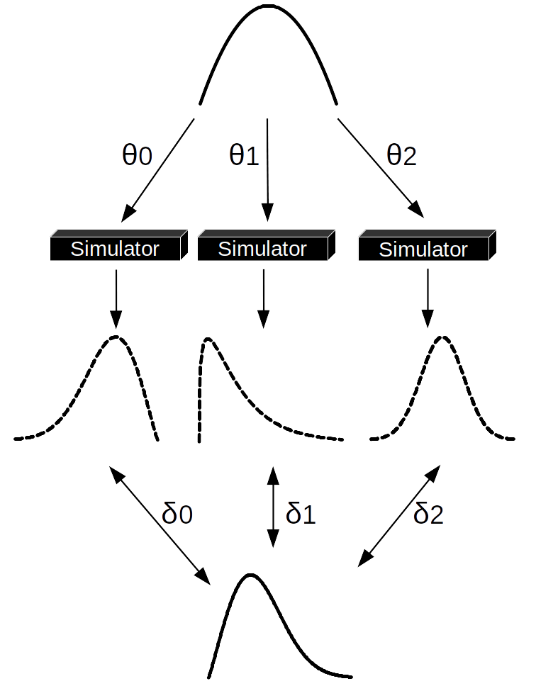
../_images/ABC_rejection.png — Fig. 8.1 One step of an ABC-rejection sampler. We sample a set of \(\theta\) values from the prior distribution (at the top). Each value is passed to the simulator, which generates synthetic datasets (dashed distributions), we compare the synthetic data with the observed one (the distribution at the bottom). In this example only \(\theta_1\) was able to generate a synthetic dataset close enough to the observed data, thus \(\theta_0\) and \(\theta_2\) were rejected. Notice that if we were using a summary statistics, instead of the entire dataset we should compute the summary statistics of the synthetic and observed data after step 2 and before step 3.#

The major drawback of the ABC-rejection sampler is that if the prior distribution is too different from the posterior distribution we will spend most of the time proposing values that will be rejected. A better idea is to propose from a distribution closer to the actual posterior. Generally we do not know enough about the posterior to do this by hand, but we can achieve it using a Sequential Monte Carlo (SMC) method. This is a general sampler method, like the MCMC methods we have been using in the book. SMC can be adapted to perform ABC and then it is called SMC-ABC. If you want to learn more about the detail of the SMC method you can read Section Inference Methods, but to understand this chapter you just need to know that SMC proceeds by increasing the value of a auxiliary parameter \(\beta\) in \(s\) successive stages \(\{\beta_0=0 < \beta_1 < ... < \beta_s=1\}\). This is done in such a way that we start sampling from the prior (\(\beta = 0\)) until we reach the posterior (\(\beta = 1\)). Thus, we can think of \(\beta\) as a parameter that gradually turns the likelihood on. The intermediate values of \(\beta\) are automatically computed by SMC. The more informative the data with respect to the prior and/or the more complex the geometry of the posterior the more intermediate steps SMC will take. Fig. 8.2 shows an hypothetical sequence of intermediate distributions from the prior in light grey to the posterior in blue.

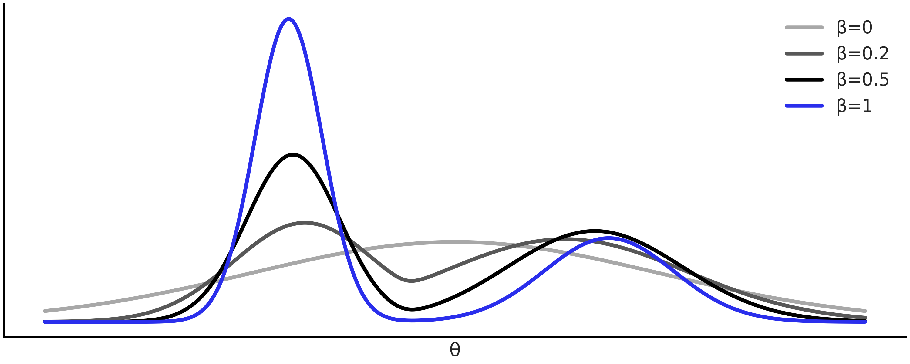
../_images/smc_tempering.png — Fig. 8.2 Hypothetical sequence of tempered posteriors explored by an SMC sampler, from the prior (\(\beta = 0\)), light gray, to the actual posterior (\(\beta = 1\)), blue. Low \(\beta\) values at the beginning helps the sampler to not get stuck in a single maximum.#

8.3. Fitting a Gaussian the ABC-way#

Let us warm up with a simple example, the estimation of the mean and standard deviation from Gaussian distributed data with mean 0 and standard deviation 1. For this problem we can fit the model:

(8.5)#\[ \begin{align}\begin{aligned}\begin{split}\begin{split} \boldsymbol{\mu} \sim &\; \mathcal{N}(0, 1) \\ \boldsymbol{\sigma} \sim &\; \mathcal{HN}(1) \\ \boldsymbol{s} \sim &\; \mathcal{N}(\boldsymbol{\mu}, \boldsymbol{\sigma})\end{split}\\\end{split}\end{aligned}\end{align} \]

The straightforward way to write this model in PyMC3 is shown in Code Block gauss_nuts.

Listing 8.1 gauss_nuts#

with pm.Model() as gauss:
    μ = pm.Normal("μ", mu=0, sigma=1)
    σ = pm.HalfNormal("σ", sigma=1)
    s = pm.Normal("s", μ, σ, observed=data)
    trace_g = pm.sample()

The equivalent model using SMC-ABC is shown in Code Block gauss_abc.

Listing 8.2 gauss_abc#

with pm.Model() as gauss:
    μ = pm.Normal("μ", mu=0, sigma=1)
    σ = pm.HalfNormal("σ", sigma=1)
    s = pm.Simulator("s", normal_simulator, params=[μ, σ],
                     distance="gaussian",
                     sum_stat="sort",  
                     epsilon=1,
                     observed=data)
    trace_g = pm.sample_smc(kernel="ABC")

We can see there are two important differences between Code Block gauss_nuts and Code Block gauss_abc:

The use of the pm.Simulator distribution
The use of pm.sample_smc(kernel="ABC") instead of pm.sample().

By using pm.Simulator we are telling PyMC3 that we are not going to use a closed form expression for the likelihood, and instead we are going to define a pseudo-likelihood. We need to pass a Python function that generates synthetic data, in this example the function normal_simulator, together with its parameters. Code Block normal_simulator shows the definition of this function for a sample size of 1000 and unknown parameters \(\mu\) and \(\sigma\).

Listing 8.3 normal_simulator#

def normal_simulator(μ, σ):
    return np.random.normal(μ, σ, 1000)

We may also need to pass other, optional, arguments to pm.Simulator including the distance function distance, the summary statistics sum_stat and the value of the tolerance parameter \(\epsilon\) epsilon. We will discuss these arguments in detail later. We also pass the observed data to the simulator distribution as with a regular likelihood.

By using pm.sample_smc(kernel="ABC")[3] we are telling PyMC3 to look for a pm.Simulator in the model and use it to define a pseudo-likelihood, the rest of the sampling process is the same as the one described for the SMC algorithm. Other samplers will fail to run when pm.Simulator is present.

The final ingredient is the normal_simulator function. In principle we can use whatever Python function we want, in fact we can even wrap non-Python code, like Fortran or C code. That is where the flexibility of ABC methods reside. In this example our simulator is just a wrapper around a NumPy random generator function.

As with other samplers it is recommended that we run more than one chain so we can diagnose if the sampler failed to work properly, PyMC3 will try to do this automatically. Fig. 8.3 shows the result of running Code Block gauss_abc with two chains. We can see that we were able to recover the true parameters and that the sampler is not showing any evident sampling issue.

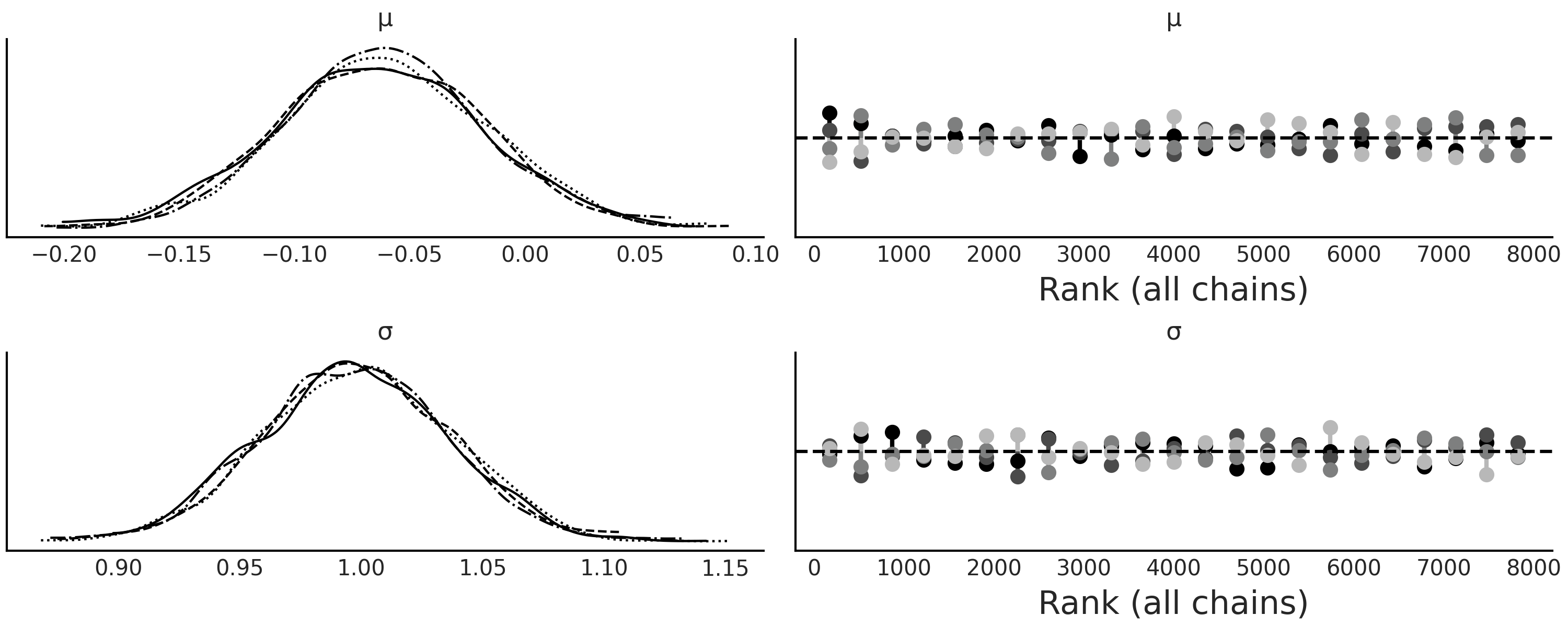
../_images/trace_g.png — Fig. 8.3 As expected \(\mu \approx 0\) and \(\sigma \approx 1\), both chains agree about the posterior as reflected by the KDEs and also by the rank plots. Notice that each of these 2 chains was obtained by running 2000 parallel SMC-chains/particles as described in the SMC algorithm.#

8.4. Choosing the Distance Function, \(\epsilon\) and the Summary Statistics#

Defining a useful distance, summary statistic and \(\epsilon\) is problem dependent. This means that we should expect some trial and error before getting good results, especially when jumping into a new problem. As usual thinking first about good options helps to reduce the number of choices. But we should embrace running experiments too as they are always helpful to better understand the problem and to make a more informed decision about these hyperparameters. In the following sections we will discuss a few general guidelines.

8.4.1. Choosing the Distance#

We run Code Block gauss_abc with the default distance function distance="gaussian", which is defined as:

(8.6)#\[\sum_i - \frac{||X_{oi} - X_{si}||^2}{2 \epsilon_i^2}\]

Where \(X_{o}\) is the observed data, \(X_{s}\) is the simulated data and \(\epsilon\) its scaling parameter. We call (8.6) Gaussian because it is the Gaussian kernel[4] in log scale. We use the log scale to compute pseudo-likelihood as we did with actual likelihoods (and priors)[5]. \(||X_{oi} - X_{si}||^2\) is the Euclidean distance (also known as L2 norm) and hence we can also describe Equation (8.6) as a weighted Euclidean distance. This is a very popular choice in the literature. Other popular options are the L1 norm (the sum of absolute differences), called Laplace distance in PyMC3, the L\(\infty\) norm (the maximum absolute value of the differences) or the Mahalanobis distance: \(\sqrt{(xo - xs)^{T}\Sigma(xo - xs)}\), where \(\Sigma\) is a covariance matrix.

Distances such as Gaussian, Laplace, etc can be applied to the whole data or, as we already mentioned, to summary statistics. There are also some distance functions that have been introduced specifically to avoid the need of summary statistics and still provide good results [92, 93, 94]. We are going to discuss two of them, the Wasserstein distances and the KL divergence.

In Code Block gauss_abc we use sum_stat="sort" [6], this tells PyMC3 to sort the data before computing Equation (8.6). Doing this is equivalent to computing the 1D 2-Wasserstein distance and if we do the same but we use the L1 norm we get the 1D 1-Wasserstein distance. It is possible to define Wasserstein distances for dimensions larger than 1 [94].

Sorting the data before computing the distance makes the comparison between distributions much more fair. To see this imagine we have two samples that are exactly equal, but out of pure luck one is ordered from low to high and the other from high to low. In such a case if we apply a metric like Equation (8.6) we would conclude both samples are very dissimilar, even when they are the same sample. But if we sort first, we will conclude they are the same. This is a very extreme scenario but it helps clarify the intuition behind sorting the data. One more thing, if we sort the data we are assuming we only care about the distribution and not the order of the data, otherwise sorting will destroy the structure in the data. This could happen, for example, with a time series, see Chapter 6.

Another distance introduced to avoid the need to define a summary statistic is the use of the KL divergence (see Section Kullback-Leibler Divergence). The KL divergence is approximated using the following expression [92, 93]:

(8.7)#\[\frac{d}{n} \sum \left(- \frac{\log(\frac{\nu_d}{\rho_d})}{\epsilon} \right) + \log\left(\frac{n}{n-1}\right)\]

Where \(d\) is the dimension of the dataset (number of variables or features), \(n\) is the number of observed datapoints. \(\nu_d\) contains the 1-nearest neighbor distances of the observed to simulated data and \(\rho_d\) the 2-nearest neighbor distances of the observed data to itself (notice that if you compare a dataset with itself the 1-nearest neighbor distances will always be zero). As this method involves 2n operations of nearest neighbor search, it is generally implemented using k-d trees [95].

8.4.2. Choosing \(\epsilon\)#

In many ABC methods the \(\epsilon\) parameter works as a hard-threshold, \(\theta\) values generating samples with distance larger than \(\epsilon\) are rejected. Additionally \(\epsilon\) can be a list of decreasing values that the user has to set or the algorithm adaptive finds [7].

In PyMC3, \(\epsilon\) is the scale of the distance function, like in Equation (8.6), so it does not work as a hard-threshold. We can set \(\epsilon\) according to our needs. We can choose a scalar value (which is equivalent to setting \(\epsilon_i\) equal for all \(i\)). This is useful when evaluating the distance over the data instead of using summary statistics. In this case a reasonably educated guess could be the empirical standard deviation of the data. If we instead use a summary statistic then we can set \(\epsilon\) to a list of values. This is usually necessary as each summary statistic may have a different scale. If the scales are too different then the contribution of each summary statistic will be uneven, it may even occur that a single summary statistic dominates the computed distances. A popular choice for \(\epsilon\) in those cases is the empirical standard deviation of the \(i^{\text{th}}\) summary statistic under the prior predictive distribution, or the median absolute deviation, as this is more robust to outliers. A problem with using the prior predictive distribution is that it can be way broader than the posterior predictive distribution. Thus to find a useful value of \(\epsilon\) we may want to take these educated guesses previously mentioned as upper bound and then from those values try also a few lower values. Then we could choose a final value of \(\epsilon\) based on several factors including the computational cost, the needed level of precision/error and the efficiency of the sampler. In general the lower the value of \(\epsilon\) the better the approximation. Fig. 8.4 shows a forest plot for \(\mu\) and \(\sigma\) for several values of \(\epsilon\) and also for the “NUTS” sampler (using a normal likelihood instead of a simulator).

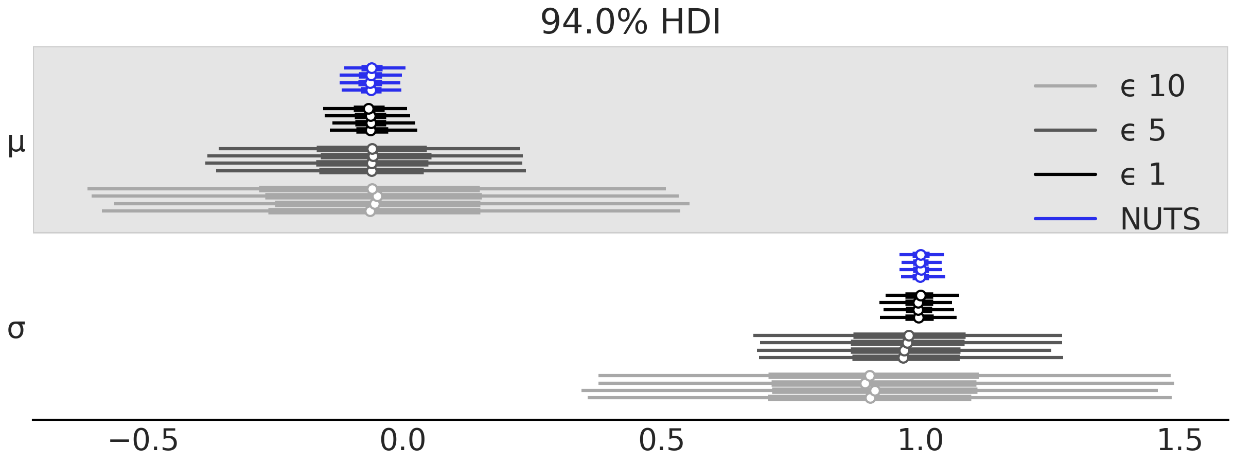
../_images/trace_g_many_eps.png — Fig. 8.4 Forest plot for \(\mu\) and \(\sigma\), obtained using NUTS or ABC with increasing values of \(\epsilon\), 1, 5, and 10.#

Decreasing the value of \(\epsilon\) has a limit, a too low value will make the sampler very inefficient, signaling that we are aiming at an accuracy level that does not make too much sense. Fig. 8.5 shows how the SMC sampler fails to converge when the model from Code Block gauss_abc is sampled with a value of epsilon=0.1. As we can see the sampler fails spectacularly.

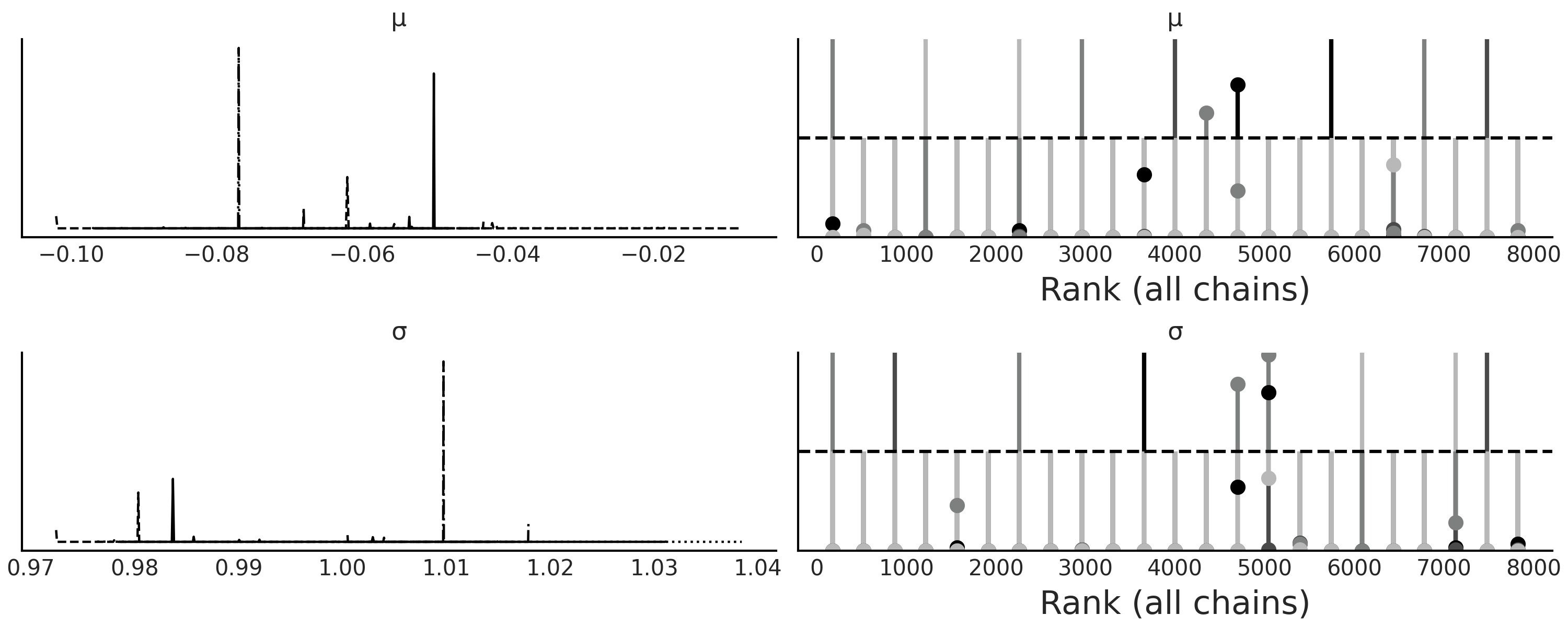
../_images/trace_g_eps_too_low.png — Fig. 8.5 KDE and rank plot for model `trace_g_001`, failure of convergence could indicate that the value \(\epsilon=0.1\) is too low for this problem.#

To help us decide on a good value for \(\epsilon\) we can get help from the model criticism tools we have been using for non-ABC methods, like Bayesian p-values and posterior predictive checks as exemplified in Figures Fig. 8.6, Fig. 8.7, and Fig. 8.8. Fig. 8.6 includes the value \(\epsilon=0.1\). We do that here to show what poorly calibrated models look like. But in practice if we obtain a rank plot like the one in Fig. 8.5 we should stop right there with the analysis of the computed posterior and reinspect the model definition. Additionally, for ABC methods, we should also inspect the value of the hyperparameter \(\epsilon\), the summary statistics we have chosen or the distance function.

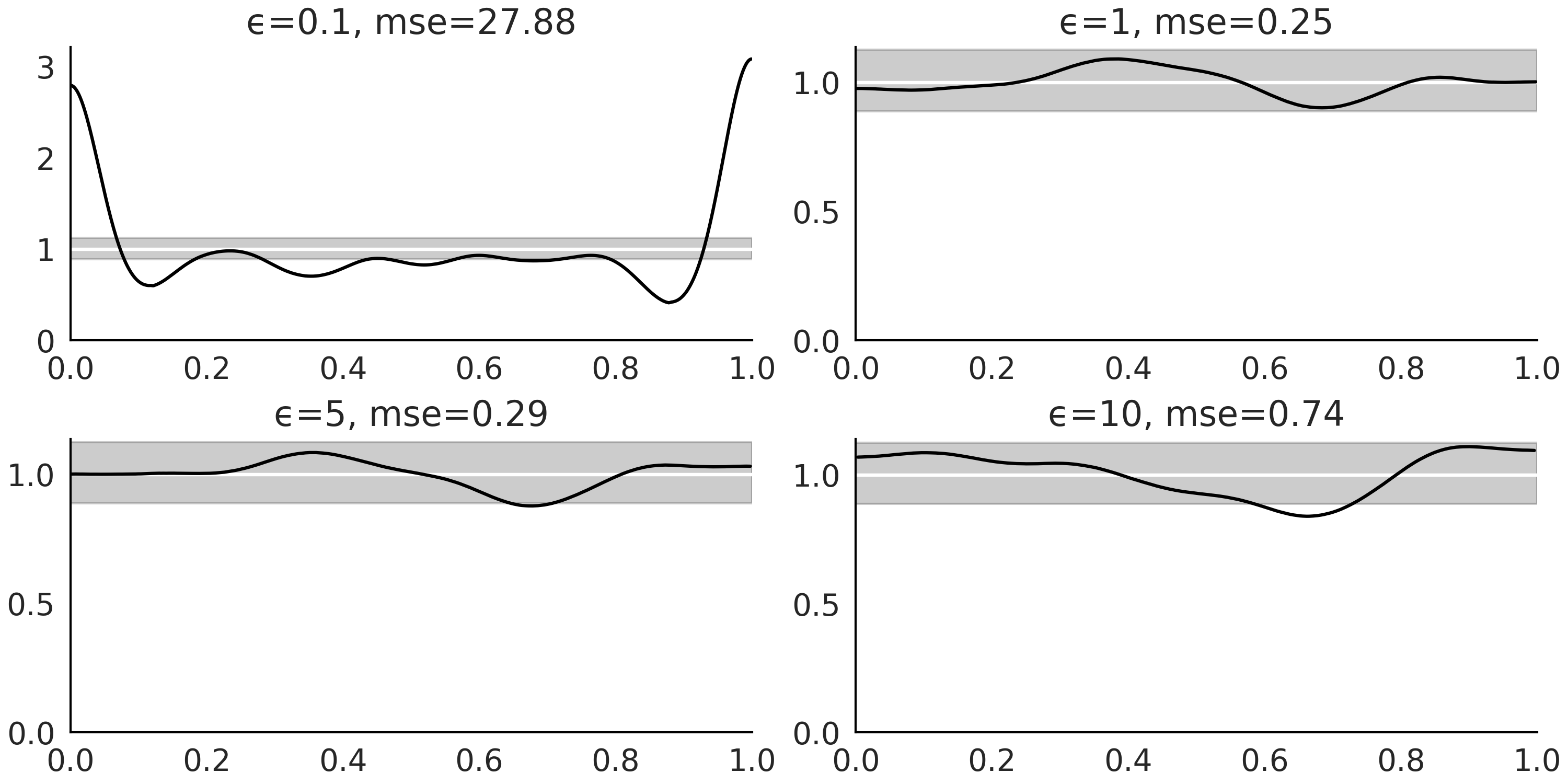
../_images/bpv_g_many_eps_00.png — Fig. 8.6 Distribution of marginal Bayesian p-values for increasing values of \(\epsilon\). For a well calibrated model we should expect a Uniform distribution. We can see that for \(\epsilon=0.1\) the calibration is terrible, this is not surprising as this value of \(\epsilon\) is too. For all the other values of \(\epsilon\) the distribution looks much more Uniform and the level of uniformity decreases as \(\epsilon\) increases. The `se` values are the (scaled) squared differences between the expected Uniform distribution and the computed KDEs.#

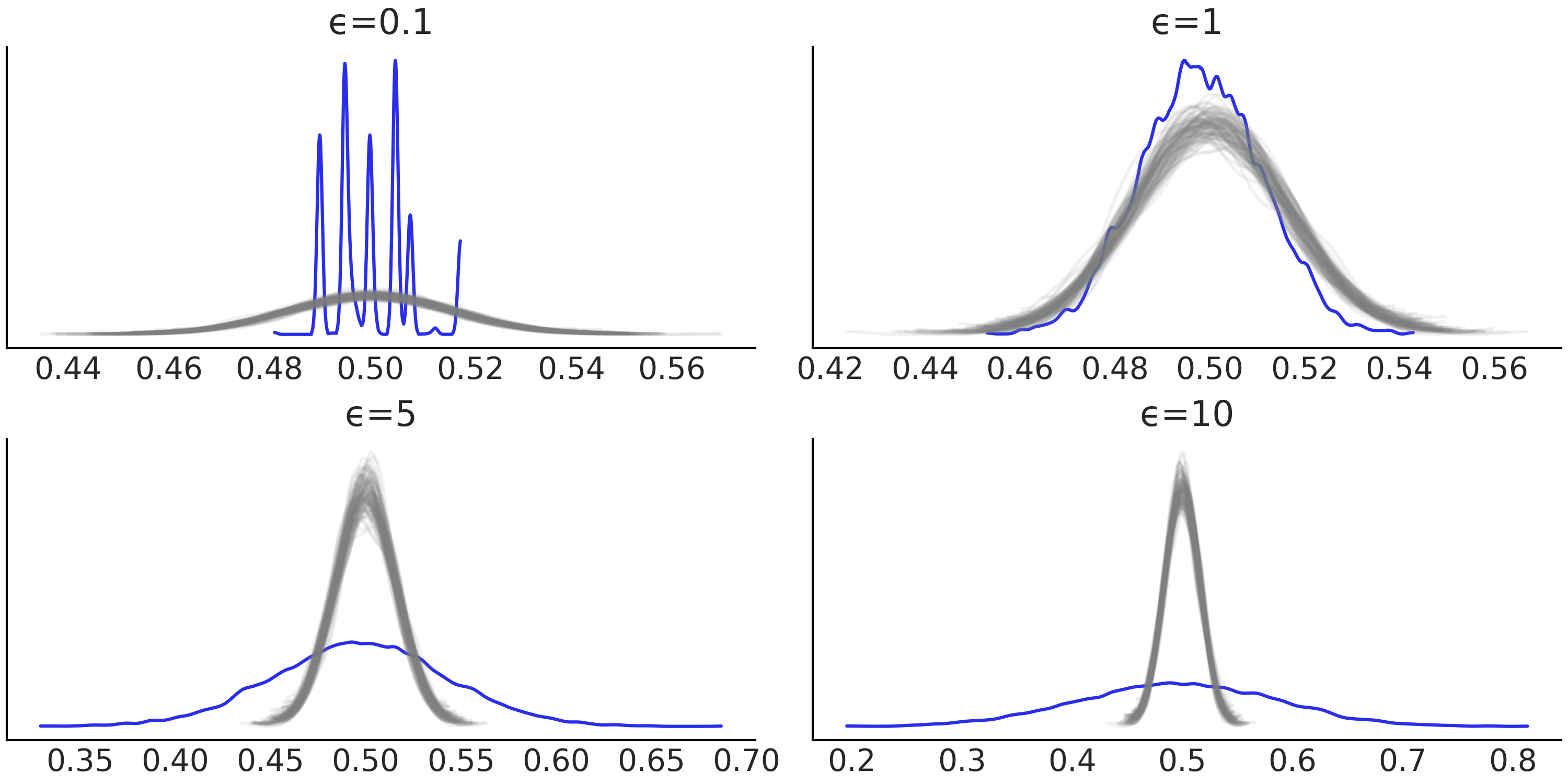
../_images/bpv_g_many_eps_01.png — Fig. 8.7 Bayesian p-values for increasing values of epsilon. The blue curve is the observed distribution and the gray curves the expected ones. For a well calibrated model we should expect a distribution concentrated around 0.5. We can see that for \(\epsilon=0.1\) the calibration is terrible, this is not surprising as this value of \(\epsilon\) is too low. We can see that \(\epsilon=1\) provides the best results.#

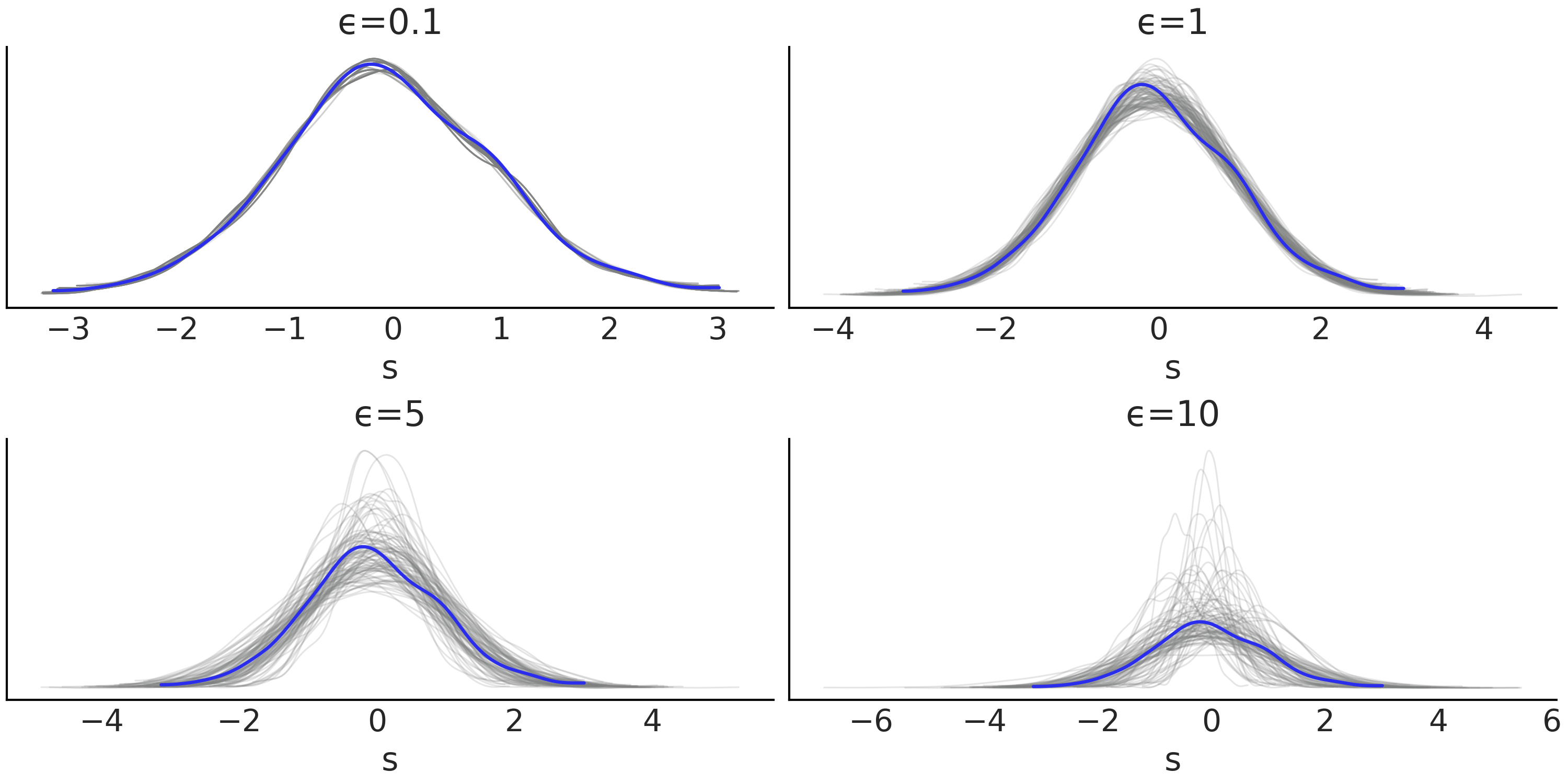
../_images/ppc_g_many_eps.png — Fig. 8.8 Posterior predictive checks for increasing values of \(\epsilon\). The blue curve is the observed distribution and the gray curves the expected ones. Surprisingly from \(\epsilon=0.1\) we get what seems to be a good adjustment, even when we know that the samples from that posterior are not trustworthy, this is a very simple example and we got the right answer out of pure luck. This is an example of *a too good to be true fit*. These are the worst! If we only consider models with posterior samples that look reasonable (i.e. not \(\epsilon=0.1\) ), we can see that \(\epsilon=1\) provides the best results.#

8.4.3. Choosing Summary Statistics#

The choice of summary statistics is arguably more difficult and will have a larger effect than the choice of the distance function. For that reason a lot of research has been focused on the subject from the use of distance that does not require summary statistics [93, 94] to strategies for choosing summary statistics [96].

A good summary statistic provides a balance between low dimension and informativeness. When we do not have a sufficient summary statistic it is tempting to overcompensate by adding a lot of summary statistics. The intuition is that the more information the better. However, increasing the number of summary statistics can actually reduce the quality of the approximated posterior [96]. One explanation for this is that we move from computing distances over data to distances over summaries to reduce the dimensionality, by increasing the number of summaries statistics we are defeating that purpose.

In some fields like population genetics, where ABC methods are very common, people have developed a large collection of useful summary statistics [97, 98, 99]. In general it is a good idea to check the literature from the applied field you are working on to see what others are doing, as chances are high they have already tried and tested many alternatives.

When in doubt we can follow the same recommendations from the previous section to evaluate the model fit, i.e rank plots, Bayesian p-values, posterior predictive checks, etc and try alternatives if necessary (see Figures Fig. 8.5, Fig. 8.6, Fig. 8.7, and Fig. 8.8).

8.5. g-and-k Distribution#

Carbon monoxide (CO) is a colorless, odorless gas that can be harmful, even fatal, when inhaled in large amounts. This gas is generated when something is burned, especially in situations when oxygen levels are low. CO together with other gases like Nitrogen Dioxide (NO₂) are usually monitored in many cities around the world to assess the level of air pollution and the quality of air. In a city the main sources of CO are cars, and other vehicles or machinery that work by burning fossil fuels. Fig. 8.9 shows a histogram of the daily CO levels measured by one station in the city of Buenos Aires from 2010 to 2018. As we can see the data seems to be slightly right skewed. Additionally the data present a few observations with very high values. The bottom panel omits 8 observations between 3 and 30.

../_images/co_ppm_bsas.png — Fig. 8.9 Histogram of CO levels. The top panel shows the entire data and the bottom one omits values larger than 3.#

To fit this data we are going to introduce the univariate g-and-k distribution. This is a 4 parameter distribution able to describe data with high skewness and/or kurtosis [100, 101]. Its density function in unavailable in closed form and the g-and-k distribution are defined through its quantile function, i.e. the inverse of the cumulative distribution function:

(8.8)#\[a + b \ \left(1 + c \ \text{tanh}\left[\frac{gz(x)}{2}\right]\right) \left(1+z(x)^2\right)^k z(x)\]

where \(z\) is the inverse of the standard normal cumulative distribution function and \(x \in (0,1)\).

The parameters \(a\), \(b\), \(g\) and \(k\) are the location, scale, skewness and kurtosis parameters respectively. If \(g\) and \(k\) are 0, we recover the Gaussian distribution with mean \(a\) and standard deviation \(b\). \(g > 0\) gives positive (right) skewness and \(g < 0\) gives negative (left) skewness. The parameter \(k \geqslant 0\) gives longer tails than the normal and \(k < 0\) gives shorter tails than the normal. \(a\) and \(g\) can take any real value. It is common to restrict \(b\) to be positive and \(k \geqslant -0.5\) or sometimes \(k \geqslant 0\) i.e. tails as heavy or heavier than those from a Gaussian distribution. Additionally it is common to fix \(c=0.8\). With all these restrictions we are guaranteed to get a strictly increasing quantile function [101] which is a hallmark of well-defined continuous distribution functions.

Code Block gk_quantile defines a g-and-k quantile distribution. We have omitted the calculation of the cdf and pdf because they are a little bit more involved, but most importantly because we are not going to use them for our examples [8]. While the probability density function of the g-and-k distribution can be evaluated numerically [101, 102], simulating from the g-and-k model using the inversion method is more straightforward and fast [102, 103]. To implement the inversion method we sample \(x \sim \mathcal{U}(0, 1)\) and replace in Equation (8.8). Code Block gk_quantile shows how to do this in Python and Fig. 8.10 shows examples of g-and-k distributions.

Listing 8.4 gk_quantile#

class g_and_k_quantile:
    def __init__(self):
        self.quantile_normal = stats.norm(0, 1).ppf

    def ppf(self, x, a, b, g, k):
        z = self.quantile_normal(x)
        return a + b * (1 + 0.8 * np.tanh(g*z/2)) * ((1 + z**2)**k) * z

    def rvs(self, samples, a, b, g, k):
        x = np.random.normal(0, 1, samples)
        return ppf(self, x, a, b, g, k)

../_images/gk_quantile.png — Fig. 8.10 The first row shows the quantile function, also known as the inverse of the cumulative distribution function. You feed it with a quantile value and it returns the value of the variable that represents that quantile. For example, if you have \(P(X <= x_q) = q\), you pass \(q\) to the quantile function and you get \(x_q\). The second row shows the (approximated) pdf. For this example the pdf has been computed using a kernel density estimation from the random samples generated with Code Block gk_quantile.#

To fit a g-and-k distribution using SMC-ABC, we can use the Gaussian distance and sum_stat="sort" as we did for the Gaussian example. Alternative, we can also think of a summary statistic tailored for this problem. As we know, the parameters \(a\), \(b\), \(g\) and \(k\) are associated with location, scale, skewness and kurtosis respectively. Thus, we can think of a summary statistic based on robust estimates for these quantities [103]:

(8.9)#\[\begin{split}\begin{split} sa &= e4 \\ sb &= e6 - e2 \\ sg &= (e6 + e2 - 2*e4)/sb \\ sk &= (e7 - e5 + e3 - e1)/sb \\ \end{split}\end{split}\]

where \(e1\) to \(e7\) are octiles, i.e. the quantiles that divide a sample into eight subsets.

If we pay attention we can see that \(sa\) is the median and \(sb\) the interquartile range, which are robust estimators of location and dispersion. Even when \(sg\) and \(sk\) may look a little bit more obscure, they are also robust estimators of skewness [104] and kurtosis [105], respectively. Let us make this more clear. For a symmetric distribution \(e6-e4\) and \(e2-e4\) will have the same magnitude but opposite signs so in such a case \(sg\) will be zero, and for skewed distributions either \(e6-e4\) will be larger than \(e2-e4\) or vice versa. The two terms in the numerator of \(sk\) increase when the mass in the neighbourhood of \(e6\) and \(e2\) decreases, i.e. when we move mass from the central part of the distribution to the tails. The denominator in both \(sg\) and \(sk\) acts as a normalization factor.

With this idea in mind we can use Python to create a summary statistic for our problem as specified in the following code block.

def octo_summary(x):
    e1, e2, e3, e4, e5, e6, e7 = np.quantile(
        x, [.125, .25, .375, .5, .625, .75, .875])
    sa = e4
    sb = e6 - e2
    sg = (e6 + e2 - 2*e4)/sb
    sk = (e7 - e5 + e3 - e1)/sb
    return np.array([sa, sb, sg, sk])

Now we need to define a simulator, we can just wrap the rvs method from the g_and_k_quantile() function previously defined in Code Block gk_quantile.

gk = g_and_k_quantile()
def gk_simulator(a, b, g, k):
    return gk.rvs(len(bsas_co), a, b, g, k)

Having defined the summary statistic and the simulator and having imported the data, we can define our model. For this example we use weakly informative priors based on the fact that all the parameters are restricted to be positive. CO levels can not take negative values so \(a\) is positive and \(g\) is also expected to be 0 or positive as most common levels are expected to be “low”, with some measurement taking larger values. We also have reasons to assume that the parameters are most likely to be below 1.

with pm.Model() as gkm:
    a = pm.HalfNormal("a", sigma=1)
    b = pm.HalfNormal("b", sigma=1)
    g = pm.HalfNormal("g", sigma=1)
    k = pm.HalfNormal("k", sigma=1)
    
    s = pm.Simulator("s", gk_simulator,
    params=[a, b, g, k],        
                     sum_stat=octo_summary,
                     epsilon=0.1,
                     observed=bsas_co)
    
    trace_gk = pm.sample_smc(kernel="ABC", parallel=True)

Fig. 8.11 shows a pair plot of the fitted gkm model.

../_images/pair_gk.png — Fig. 8.11 The distribution is slightly skewed and with some degree of kurtosis as expected from the few CO levels with values one or two orders of magnitude larger than the bulk of CO values. We can see that \(b\) and \(k\) are (slightly) correlated. This is expected, as the density in the tail (kurtosis) increases, the dispersion increases, but the g-and-k distribution can keep \(b\) small if \(k\) increases. It is like \(k\) is *absorbing* part of the dispersion, similar to what we observed with the scale and the \(\nu\) parameter in a Student’s t-distribution.#

8.6. Approximating Moving Averages#

The moving-average (MA) model is a common approach for modeling univariate time series (see Chapter 6). The MA(q) model specifies that the output variable depends linearly on the current and \(q\) previous past values of a stochastic term \(\lambda\). \(q\) is known as the order of the MA model.

(8.10)#\[y_t = \mu + \lambda_t + \theta_1 \lambda_{t-1} + \cdots + \theta_q \lambda_{t-q}\]

where \(\lambda\) are white Gaussian noise error terms [9].

We are going to use a toy-model taken from Marin et al. [106]. For this example we are going to use the MA(2) model with mean value 0 (i.e. \(\mu =0\)), thus our model looks like:

(8.11)#\[y_t = \lambda_t + \theta_1 \lambda_{t-1} + \theta_2 \lambda_{t-2}\]

Code Block ma2_simulator_abc shows a Python simulator for this model and in Fig. 8.12 we can see two realizations from that simulator for the values \(\theta1 = 0.6, \theta2=0.2\).

Listing 8.5 ma2_simulator_abc#

def moving_average_2(θ1, θ2, n_obs=200):
    λ = np.random.normal(0, 1, n_obs+2)
    y = λ[2:] + θ1*λ[1:-1] + θ2*λ[:-2]
    return y

../_images/ma2_simulator_abc.png — Fig. 8.12 Two realizations of a MA(2) model, one with \(\theta1=0.6, \theta2 =0.2\). On the left column the kernel density estimation on the right column the time series.#

In principle we could try to fit a MA(q) model using any distance function and/or summary statistic we want. Instead, we can use some properties of the MA(q) model as a guide. One property that is often of interest in MA(q) models is their autocorrelation. Theory establishes that for a MA(q) model the lags larger than q will be zero, so for a MA(2) seems to be reasonable to use as summary statistics the autocorrelation function for lag 1 and lag 2. Additionally, and just to avoid computing the variance of the data, we will use the auto-covariance function instead of the auto-correlation function.

def autocov(x, n=2):
    return np.array([np.mean(x[i:] * x[:-i]) for i in range(1, n+1)])

Additionally MA(q) models are non-identifiable unless we introduce a few restrictions. For a MA(1) model, we need to restrict \(-1<\theta_1<1\). For MA(2) we have \(-2<\theta_1<2\), \(\theta_1+\theta_2>-1\) and \(\theta_1-\theta_2<1\), this implies that we need to sample from a triangle as shown in Fig. 8.14.

Combining the custom summary statistics and the identifiable restrictions we have that the ABC model is specified as in Code Block MA2_abc.

Listing 8.6 MA2_abc#

with pm.Model() as m_ma2:
    θ1 = pm.Uniform("θ1", -2, 2)
    θ2 = pm.Uniform("θ2", -1, 1)
    p1 = pm.Potential("p1", pm.math.switch(θ1+θ2 > -1, 0, -np.inf))
    p2 = pm.Potential("p2", pm.math.switch(θ1-θ2 < 1, 0, -np.inf))

    y = pm.Simulator("y", moving_average_2, 
                     params=[θ1, θ2],
                     sum_stat=autocov,
                     epsilon=0.1,
                     observed=y_obs)

    trace_ma2 = pm.sample_smc(3000, kernel="ABC")

A pm.Potential is a way to incorporate arbitrary terms to a (pseudo)-likelihood, without adding new variables to the model. It is specially useful to introduce restrictions, like in this example. In Code Block MA2_abc we sum 0 to the likelihood if the first argument in pm.math.switch is true or \(-\infty\) otherwise.

../_images/ma2_trace.png — Fig. 8.13 ABC trace plot for the MA(2) model. As expected the true parameters are recovered and the rank plots look satisfactorily flat.#

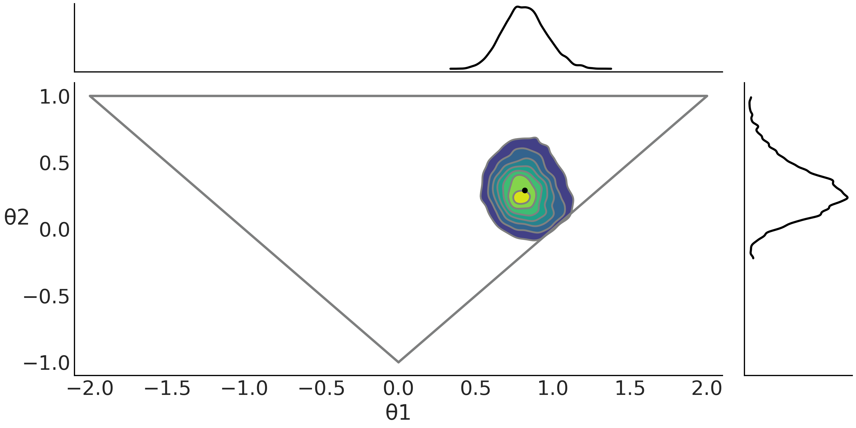
../_images/ma2_triangle.png — Fig. 8.14 ABC posterior for the MA(2) model as defined in Code Block MA2_abc. In the center subplot the joint posterior and in the margins the marginal distributions for \(\theta1\) and \(\theta2\). The gray triangle represents the prior distribution. The mean is indicated with a black dot.#

8.7. Model Comparison in the ABC Context#

ABC methods are frequently used for model choice. While many methods have been proposed [96, 107], here we will discuss two approaches; Bayes factors, including a comparison with LOO, and random forest [99].

As with parameter inference, the choice of summaries is of crucial importance for model comparison. If we evaluate two or more models using their predictions, we can not favour one model over the other if they all make roughly the same predictions. The same reasoning can be applied to model choice under ABC with summary statistics. If we use the mean as the summary statistic, but models predict the same mean, then this summary statistic will not be sufficient to discriminate between models. We should take more time to think about what makes models different.

8.7.1. Marginal Likelihood and LOO#

One common quantity used to perform model comparison for ABC methods is the marginal likelihood. Generally such comparison takes the form of a ratio of marginal likelihoods, which is known as Bayes factors. If the value of a Bayes factor is larger than 1, the model in the numerator is preferred over the one in the denominator and vice versa. In Section Marginal Likelihood and Model Comparison we discuss more details about Bayes factors, including their caveats. One such caveat is that the marginal likelihood is generally difficult to compute. Fortunately, SMC methods and by extension SMC-ABC methods are able to compute the marginal likelihood as a byproduct of sampling. PyMC3’s SMC computes and saves the log marginal likelihood in the trace. We can access its value by doing trace.report.log_marginal_likelihood. As this value is in a log scale, to compute a Bayes factor we can do:

ml1 = trace_1.report.log_marginal_likelihood
ml2 = trace_2.report.log_marginal_likelihood
np.exp(ml1 - ml2)

When using summary statistics the marginal likelihood computed from ABC methods cannot be generally trusted to discriminate between competing models [108], unless the summary statistics are sufficient for model comparison. This is worrisome as, outside a few formal examples or particular models, there is no general guide to ensure sufficiency across models [108]. This is not a problem if we use all the data i.e. we do not rely on summary statistics [10]. This resembles our discussion (see Section Marginal Likelihood and Model Comparison) about how computing the marginal likelihood is generally a much more difficult problem that computing the posterior. Even if we manage to find a summary statistic that is good enough to compute a posterior, that is not a guarantee it will be also useful for model comparison.

To better understand how the marginal likelihood behaves in the context of ABC methods we will now analyze a short experiment. We also include LOO, as we consider LOO an overall better metric than the marginal likelihood and thus Bayes factors.

The basic setup of our experiment is to compare the values of the log marginal likelihood and the values computed using LOO for models with an explicit likelihood against values from ABC models using a simulator with and without summary statistics. The results are shown in Figures Fig. 8.15 models in Code Blocks gauss_nuts and gauss_abc. The values of the marginal (pseudo)likelihood are computed as by products of SMC and the values of LOO using az.loo(). Notice that LOO is properly defined on the pointwise log-likelihood values, but in ABC we only have access to the pointwise log-pseudolikelihood values.

From Fig. 8.15 we can see that in general both LOO and the log marginal likelihood behave similarly. From the first column we see that model_1 is consistently chosen as better than model_0 (here higher is better). The difference between models (the slopes) is larger for the log marginal likelihood than for LOO, this can be explained as the computation of the marginal likelihood explicitly takes the prior into account while LOO only does it indirectly through the posterior (see Section Marginal Likelihood and Model Comparison for details). Even when the values of LOO and the marginal likelihood vary across samples they do it in a consistent way. We can see this from the slopes of the lines connecting model_0 and model_1. While the slopes of the lines are not exactly the same, they are very similar. This is the ideal behavior of a model selection method. We can reach similar conclusions if we compare model_1 and model_2. With the additional consideration that both models are basically indistinguishable for LOO, while the marginal likelihood reflects a larger difference. Once again the reason is that LOO is computed just from the posterior while the marginal likelihood directly takes the prior into account.

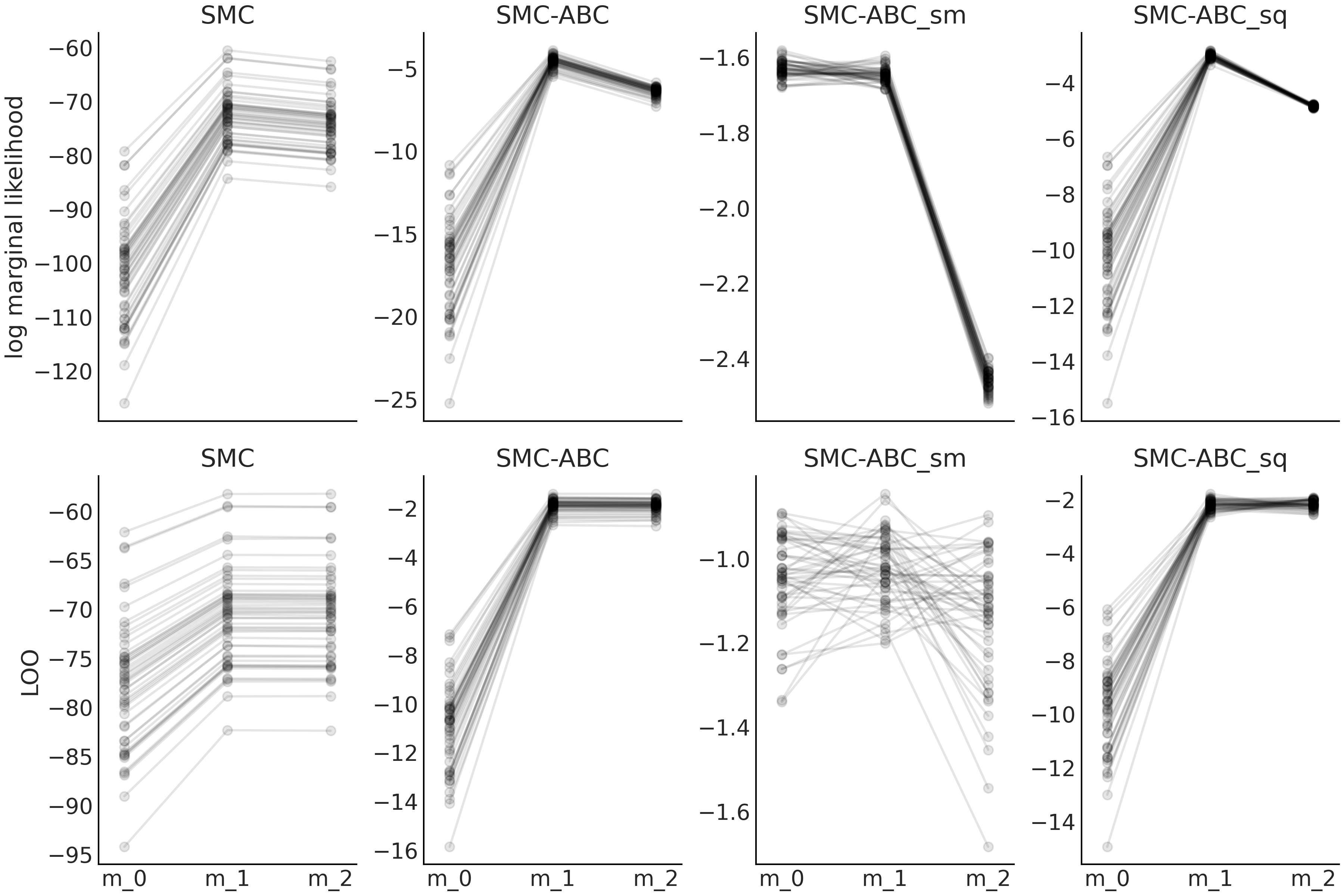
../_images/model_comp_normal_00.png — Fig. 8.15 Model `m_0` is similar as the model described in Equation (8.5) but with \(\sigma \sim \mathcal{HN}(0.1)\). `model_1` the same as Equation (8.5). `model_2` is the same as Equation (8.5) but with \(\sigma \sim \mathcal{HN}(10)\). The first row corresponds to values of the log marginal likelihood and the second row to values computed using LOO. Sequential Monte Carlo `SMC`, SMC-ABC with the entire dataset `SMC-ABC`, SMC-ABC using the mean as summary statistic `SMC-ABC_sm` and finally SMC-ABC using the mean and standard deviation `SMC-ABC_sq`. We run 50 experiments each one with sample size 50.#

The second column shows what happens when we move into the ABC realm. We still get model_1 as a better choice, but now the dispersion of model_0 is much larger than the one from model_1 or model_2. Additionally we now get lines crossing each other. Taken together, both observations seems to indicate that we still can use LOO or the log marginal likelihood to select the best model, but the values of the relative weights, like the ones computed by az.compare() or the Bayes factors will have larger variability.

The third column shows what happens when we use the mean as summary statistic. Now model model_0 and model_1 seems to be on par and model_2 looks like a bad choice. It is almost like the specular image of the previous column. This shows that when using an ABC method with summary statistics the log marginal likelihood and LOO can fail to provide a reasonable answer.

The fourth column shows what happens when we use the standard deviation in addition to the mean as summary statistic. We see than we can qualitatively recover the behavior observed when using ABC with the entire dataset (second column).

On the scale of the pseudolikelihood

Notice how the scale on the y-axes is different, especially across columns. The reason is two-fold, first when using ABC we are approximating the likelihood with a kernel function scaled by \(\epsilon\), second when using a summary statistic we are decreasing the size of the data. Notice also that this size will keep constant if we increase the sample size for summary statistics like the mean or quantiles, i.e. the mean is a single number irrespective if we compute it from 10 or 1000 observations.

Fig. 8.16 can help us to understand what we just discussed from Fig. 8.15. We recommend you analyze both figures together by yourself. For the moment we will focus on two observations. First, when performing SMC-ABC_sm we have a sufficient statistics for the mean but nothing to say about the dispersion of the data, thus the posterior uncertainty of both parameters a and σ is essentially controlled by the prior. See how the estimates from model_0 and model_1 are very similar for μ and the uncertainty from model_2 is ridiculously large. Second, and regarding the parameter σ the uncertainty is very small for model_0, wider that it should be for model_1 and ridiculously large for model_2. Taken all together we can see why the log marginal likelihood and LOO indicate that model_0 and model_1 are on par but model_2 is very different. Basically, SMC-ABC_sm is failing to provide a good fit! Once we see this is no longer surprising that the log marginal likelihood and LOO computed from SMC-ABC_sm contradicts what is observed when we use SMC or SMC-ABC. If we use the mean and the standard deviation SMC-ABC_sq as summary statistics we partially recover the behavior of using the whole data-set SMC-ABC.

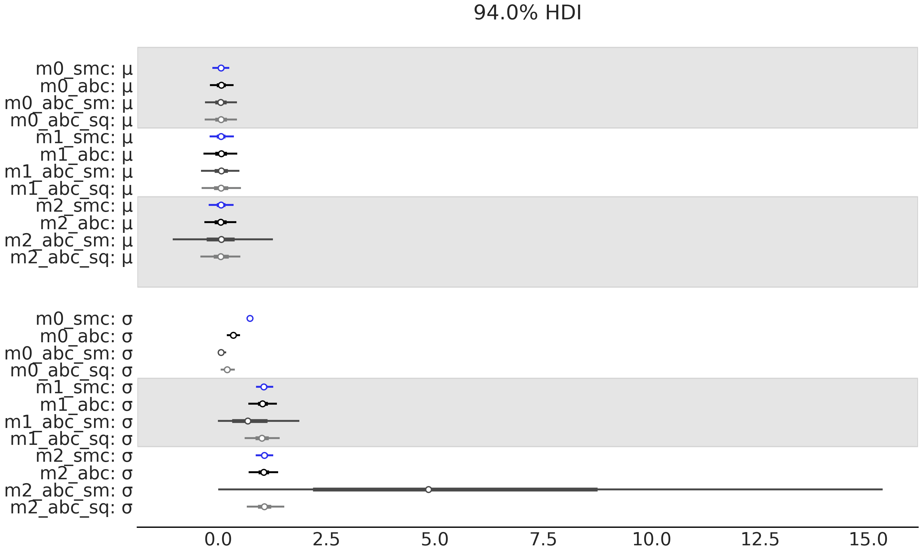
../_images/model_comp_normal_forest.png — Fig. 8.16 Model `m_0` is similar as the model described in Equation (8.5) but with \(\sigma \sim \mathcal{HN}(0.1)\). `model_1` the same as Equation (8.5). `model_2` is the same as Equation (8.5) but with \(\sigma \sim \mathcal{HN}(10)\). The first row contains the values of the marginal likelihood and the second the values of LOO. The column represents different methods of computing these values. Sequential Monte Carlo `SMC`, SMC-ABC with the entire dataset `SMC-ABC`, SMC-ABC using the mean as summary statistic `SMC-ABC_sm` and finally SMC-ABC using the mean and standard deviation `SMC-ABC_sq`. We run 50 experiments each one with sample size 50.#

Figures Fig. 8.17 and Fig. 8.18 shows a similar analysis but model_0 is a geometric model and model_1 is a Poisson model. The data follows a shifted Poisson distribution \(\mu \sim 1 + \text{Pois}(2.5)\). We leave the analysis of these figures as an exercise for the readers.

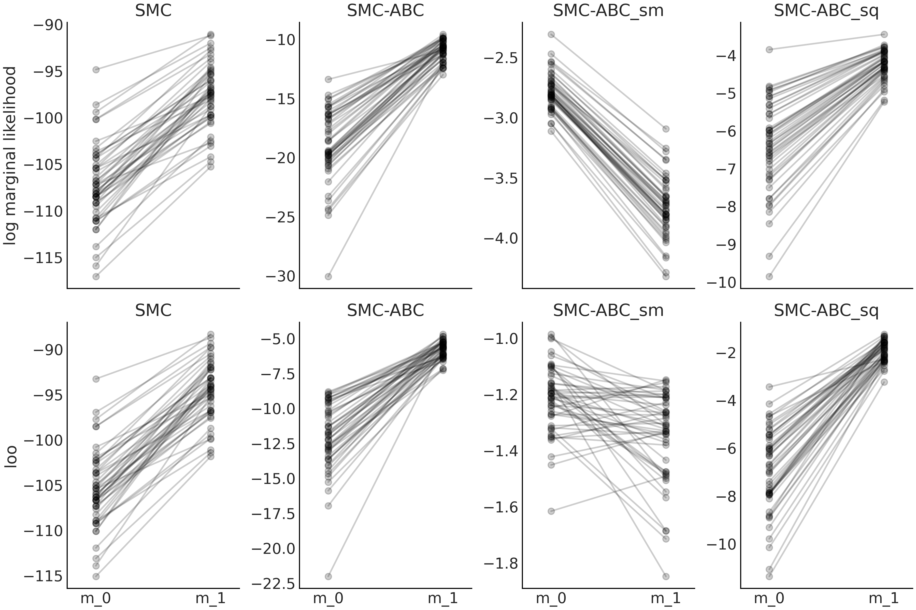
../_images/model_comp_pois_geom_00.png — Fig. 8.17 Model `m_0` is a geometric distribution with prior \(p \sim \mathcal{U}(0, 1)\) and `model_1` is a Poisson distribution with prior \(\mu \sim \mathcal{E}(1)\). The data follows a shifted Poisson distribution \(\mu \sim 1 + \text{Pois}(2.5)\). Sequential Monte Carlo `SMC`, SMC-ABC with the entire dataset `SMC-ABC`, SMC-ABC using the mean as summary statistic `SMC-ABC_sm` and finally SMC-ABC using the mean and standard deviation `SMC-ABC_sq`.We run 50 experiments each one with sample size 50.#

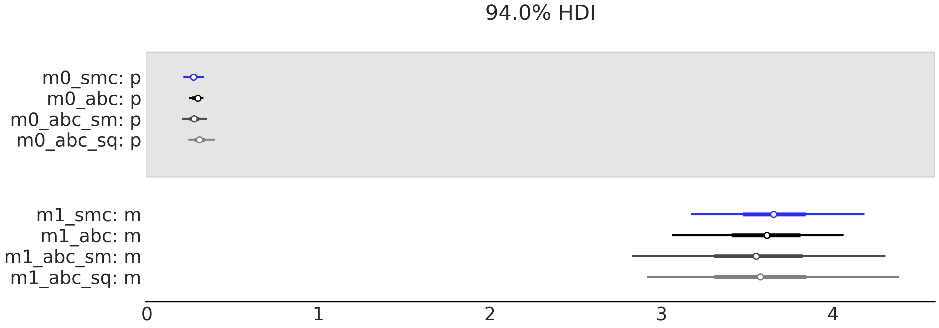
../_images/model_comp_pois_geom_forest.png — Fig. 8.18 `model_0` a geometric model/simulator with prior \(p \sim \mathcal{U}(0, 1)\) `model_1` A Poisson model/simulator with prior \(p \sim \text{Expo}(1)\). The firs row contains the values of the marginal likelihood and the second the values of LOO. The column represents different methods of computing these values. Sequential Monte Carlo `SMC`, SMC-ABC with the entire dataset `SMC-ABC`, SMC-ABC using the mean as summary statistic `SMC-ABC_sq` and finally SMC-ABC using quartiles `SMC-ABC_sq`. We run 50 experiments each one with sample size 50.#

In the ABC literature it is common to use Bayes factors in an attempt to assign relative probabilities to models. We understand this can be perceived as valuable in certain fields. So we want to warn those practitioners about the potential problems of this practice under the ABC framework, especially because it is much more common to use summary statistics than not. Model comparison can still be useful, mainly if a more exploratory approach is adopted together with model criticism performed before model comparison to improve or discard clearly misspecified models. This is the general approach we have adopted in this book for non-ABC methods so we consider natural to extend it into the ABC framework as well. In this book we also favor LOO over the marginal likelihood, while research about the benefits and drawbacks of LOO for ABC methods are currently lacking, we consider LOO to be potentially useful for ABC methods too. Stay tuned for future news!

Model criticism and model comparison

While some amount of misspecification is always expected, and model comparison can help to better understand models and their misspecification. Model comparison should be done only after we have shown the models provide a reasonable fit to the data. It does not make too much sense to compare models that are clearly a bad fit.

8.7.2. Model Choice via Random Forest#

The caveats we discussed in the previous section has motivated the research of new methods for model choice under the ABC framework. One such alternative method reframes the model selection problem as random forest classification problem [99] [11]. A random forest is a method for classification and regression based on the combination of many decision trees and it is closely related to BARTs from Chapter 7.

The main idea of this method is that the most probable model can be obtained by constructing a random forest classifier from simulations from the prior or posterior predictive distributions. In the original paper authors use the prior predictive distribution but mention that for more advanced ABC method other distributions can be used too. Here we will use the posterior predictive distribution. For each model up to \(m\) models, the simulations are ordered in a reference table (see Table 8.1). where each row is a sample from the posterior predictive distribution and each column is one out of \(n\) summary statistics. We use this reference table to train the classifier, the task is to correctly classify the models given the values of the summary statistics. It is important to note that the summary statistics used for model choice does not need to be the same used to compute the posterior. In fact it is recommended to include many summary statistics. Once the classifier is trained we feed it with the same \(n\) summary statistics we used in the reference table, but this time applied to our observed data. The predicted model by the classifier will be our best model.

Table 8.1 Reference table#
Model	\(\mathbf{S^{0}}\)	\(\mathbf{S^{1}}\)	…	\(\mathbf{S^{n}}\)
0			…
0			…
…	…	…	…	…
1			…
1			…
m			…

Additionally, we can also compute an approximated posterior probability for the best model, relative to the rest of the models. Once again, this can be done using a random forest, but this time we use a regression, with the misclassification error rate as response variable and the summary statistics in the reference table as independent variables [99].

8.7.3. Model Choice for MA Model#

Let us go back to the moving average example, this time we will focus on the following question. Is a MA(1) or MA(2) a better choice? To answer this question we will use LOO (based on the pointwise pseudo-likelihood values) and random forest. The MA(1) models looks like this

Listing 8.7 MA1_abc#

with pm.Model() as m_ma1:
    θ1 = pm.Uniform("θ1", -1, 1)
    y = pm.Simulator("y", moving_average_1,
                     params=[θ1], sum_stat=autocov, epsilon=0.1, observed=y_obs)
    trace_ma1 = pm.sample_smc(2000, kernel="ABC")

In order to compare ABC-models using LOO. We cannot directly use the function az.compare. We first to need to create an InferenceData object with a log_likelihood group as detailed in Code Block idata_pseudo [12]. The result of this comparison is summarized in Table 8.2. As expected, we can see that the MA(2) model is preferred.

Listing 8.8 idata_pseudo#

idata_ma1 = az.from_pymc3(trace_ma1)
lpll = {"s": trace_ma2.report.log_pseudolikelihood}
idata_ma1.log_likelihood = az.data.base.dict_to_dataset(lpll)

idata_ma2 = az.from_pymc3(trace_ma2)
lpll = {"s": trace_ma2.report.log_pseudolikelihood}
idata_ma2.log_likelihood = az.data.base.dict_to_dataset(lpll)

az.compare({"m_ma1":idata_ma1, "m_ma2":idata_ma2})

Table 8.2 Summary ABC-model comparison using LOO#
	rank	loo	p_loo	d_loo	weight	se	dse	warning	loo_scale
model_ma2	0	-2.22	1.52	0.00	1.0	0.08	0.00	False	log
model_ma1	1	-3.53	2.04	1.31	0.0	1.50	1.43	False	log

To use the random forest method we can use the select_model function included in the accompanying code for this book. To make this function work we need to pass a list of tuples with the PyMC3’s model names and traces, a list of summary statistics, and the observed data. Here as summary statistics we will use the first six auto-correlations. We choose these particular summary statistics for two reasons, first to show that we can use a set of summary statistics different from the one used to fit the data and second two show that we can mix useful summary statistics (the first two auto-correlations), with not very useful ones (the rest). Remember that theory says that for a MA(q) processes there are at most q auto-correlations. For complex problems, like those from population genetics it is not uncommon to use several hundreds or even tens of thousands of summary statistics [109].

from functools import partial
select_model([(m_ma1, trace_ma1), (m_ma2, trace_ma2)],
             statistics=[partial(autocov, n=6)],
             n_samples=5000,
             observations=y_obs)

select_model returns the index of the best model (starting from 0) and the estimated posterior probability for that model. For our example we get model 0 with a probability of 0.68. It is a little bit reassuring that, at least for this example, both LOO and the random forest method agree on model choice and even their relative weight.

8.8. Choosing Priors for ABC#

Not having a closed form likelihood makes it more difficult to get good models and thus ABC methods are in general more brittle than other approximations. Consequently we should be extra careful about modeling choices, including prior elicitation, and more thorough about model evaluation than when we have an explicit likelihood. These are the costs we pay for approximating the likelihood.

A more careful prior elicitation can be much more rewarding with ABC methods than with other approaches. If we lose information by approximating the likelihood we can maybe partially compensate that loss by using a more informative prior. Additionally, better priors will generally save us from wasting computational resources and time. For ABC rejection methods, where we use the prior as the sampling distribution, this is more or less evident. But it is also the case for SMC methods, specifically if the simulator are sensitive to the input parameter. For example, when using ABC to inference a ordinary differential equation, some parameter combination could be numerical challenging to simulate, resulting in extremely slow simulation. Another problem of using vague prior arise during the weighted sampling in SMC and SMC-ABC, as almost all but few samples from the prior would have extremely small weights when evaluated on the tempered posteriors. This leads to the SMC particles to become singular after just a few steps (as only few samples with large weight are selected). This phenomenon is called weight collapse, a well known issue for particle methods [110]. Good priors can help to reduce the computational cost and thus to some extent allow us to fit more complex models when we are using SMC and SMC-ABC. Beyond the general advice of more informative prior and what we have already discussed elsewhere in the book about prior elicitation/evaluation, we do not have further recommendation specific for ABC methods.

8.9. Exercises#

8E1. In your words explain how ABC is approximate? What object or quantity is approximated and how.

8E2. In the context of ABC, what is the problem that SMC is trying to solve compared to rejection sampling?

8E3. Write a Python function to compute the Gaussian kernel as in Equation (8.6), but without the summation. Generate two random samples of size 100 from the same distribution. Use the implemented function to compute the distances between those two random samples. You will get two distributions each of size 100. Show the differences using a KDE plot, the mean and the standard deviation.

8E4. What do you expect to the results to be in terms of accuracy and convergence of the sampler if in model gauss model from Code Block gauss_abc we would have used sum_stat="identity". Justify.

8E5. Refit the gauss model from Code Block gauss_abc using sum_stat="identity". Evaluate the results using:

Trace Plot
Rank Plot
\(\hat R\)
The mean and HDI for the parameters \(\mu\) and \(\sigma\).

Compare the results with those from the example in the book (i.e. using sum_stat="sort").

8E6. Refit the gauss model from Code Block gauss_abc using quintiles as summary statistics.

How the results compare with the example in the book?
Try other values for epsilon. Is 1 a good choice?

8E7. Use the g_and_k_quantile class to generate a sample (n=500) from a g-and-k distribution with parameters a=0,b=1,g=0.4,k=0. Then use the gkm model to fit it using 3 different values of \(\epsilon\) (0.05, 0.1, 0.5). Which value of \(\epsilon\) do you think is the best for this problem? Use diagnostics tools to help you answer this question.

8E8. Use the sample from the previous exercise and the gkm model. Fit the using the summary statistics octo_summary, the octile-vector (i.e. the quantiles 0.125, 0.25, 0.375, 0.5, 0.625, 0.75, 0.875) and sum_stat="sorted". Compare the results with the known parameter values, which option provides higher accuracy and lower uncertainty?

8M9. In the GitHub repository you will find a dataset of the distribution of citations of scientific papers. Use SMC-ABC to fit a g-and-k distribution to this dataset. Perform all the necessary steps to find a suitable value for "epsilon" and ensuring the model converge and results provides a suitable fit.

8M10. The Lotka-Volterra is well-know biological model describing how the number of individuals of two species change when there is a predator-prey interaction [111]. Basically, as the population of prey increase there is more food for the predator which leads to an increase in the predator population. But a large number of predators produce a decline in the number of pray which in turn produce a decline in the predator as food becomes scarce. Under certain conditions this leads to an stable cyclic pattern for both populations. In the GitHub repository you will find a Lotka-Volterra simulator with unknown parameters and the data set Lotka-Volterra_00. Assume the unknown parameters are positive. Use a SMC-ABC model to find the posterior distribution of the parameters.

8H11. Following with the Lotka-Volterra example. The dataset Lotka-Volterra_01 includes data for a predator prey with the twist that at some point a disease suddenly decimate the prey population. Expand the model to allow for a “switchpoint”, i.e. a point that marks two different predator-prey dynamics (and hence two different set of parameters).

8H12. This exercise is based in the sock problem formulated by Rasmus Bååth. The problem goes like this. We get 11 socks out of the laundry and to our surprise we find that they are all unique, that is we can not pair them. What is the total number of socks that we laundry? Let assume that the laundry contains both paired and unpaired socks, we do not have more than two socks of the same kind. That is we either have 1 or 2 socks of each kind.

Assume the number of socks follows a \(\text{NB}(30, 4.5)\). And that the proportion of unpaired socks follows a \(\text{Beta}(15, 2)\)

Generate a simulator suitable for this problem and create a SMC-ABC model to compute the posterior distribution of the number of socks, the proportion of unpaired socks, and the number of pairs.