Code 11: Appendiceal Topics

This is a reference notebook for the book Bayesian Modeling and Computation in Python

The textbook is not needed to use or run this code, though the context and explanation is missing from this notebook.

If you’d like a copy it’s available from the CRC Press or from Amazon. ``

import arviz as az
import matplotlib.pyplot as plt
import numpy as np
import pandas as pd
import pymc3 as pm
from scipy import stats

from scipy.special import binom, betaln

az.style.use("arviz-grayscale")
plt.rcParams['figure.dpi'] = 300

np.random.seed(14067)

Probability Background

Code 11.1

def die():
    outcomes = [1, 2, 3, 4, 5, 6]
    return np.random.choice(outcomes)

die()

6

Code 11.2

def experiment(N=10):
    sample = [die() for i in range(N)]

    for i in range(1, 7):
        print(f"{i}: {sample.count(i)/N:.2g}")

experiment()

1: 0
2: 0.1
3: 0.3
4: 0
5: 0.2
6: 0.4

a = 1
b = 6
rv = stats.randint(a, b+1)
x = np.arange(1, b+1)

x_pmf = rv.pmf(x)  # evaluate the pmf at the x values
x_cdf = rv.cdf(x)  # evaluate the cdf at the x values
mean, variance = rv.stats(moments="mv")

Figure 11.17

xs = (np.linspace(0, 20, 200), np.linspace(0, 1, 200), np.linspace(-4, 4, 200))
dists = (stats.expon(scale=5), stats.beta(0.5, 0.5), stats.norm(0, 1))


_, ax = plt.subplots(3, 3)

for idx, (dist, x) in enumerate(zip(dists, xs)):
    draws = dist.rvs(100000)
    data = dist.cdf(draws)
    # PDF original distribution
    ax[idx, 0].plot(x, dist.pdf(x))
    # Empirical CDF
    ax[idx, 1].plot(np.sort(data), np.linspace(0, 1, len(data)))
    # Kernel Density Estimation
    az.plot_kde(data, ax=ax[idx, 2])

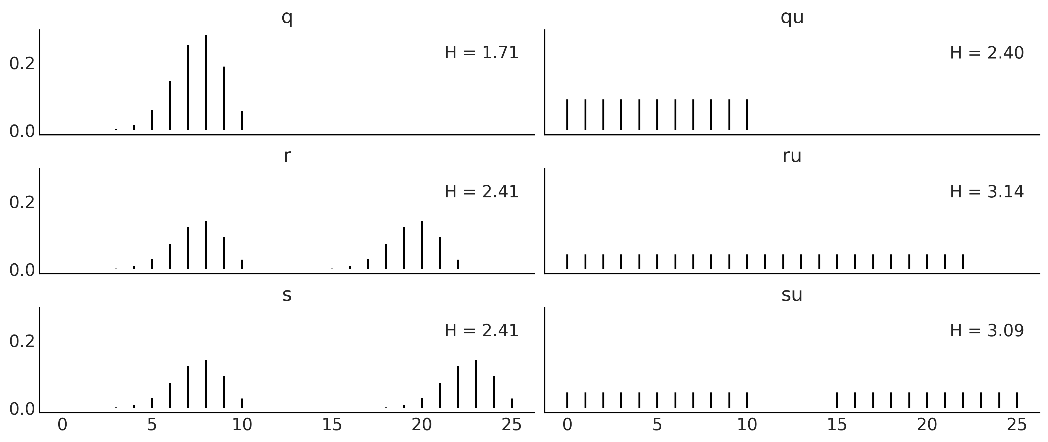
x = range(0, 26)
q_pmf = stats.binom(10, 0.75).pmf(x)
qu_pmf = stats.randint(0, np.max(np.nonzero(q_pmf))+1).pmf(x)
r_pmf = (q_pmf + np.roll(q_pmf, 12)) / 2
ru_pmf = stats.randint(0, np.max(np.nonzero(r_pmf))+1).pmf(x)
s_pmf = (q_pmf + np.roll(q_pmf, 15)) / 2
su_pmf = (qu_pmf + np.roll(qu_pmf, 15)) / 2

_, ax = plt.subplots(3, 2, figsize=(12, 5), sharex=True, sharey=True,
                     constrained_layout=True)
ax = np.ravel(ax)

zipped = zip([q_pmf, qu_pmf, r_pmf, ru_pmf, s_pmf, su_pmf],
             ["q", "qu", "r", "ru", "s", "su"])
for idx, (dist, label) in enumerate(zipped):
    ax[idx].vlines(x, 0, dist, label=f"H = {stats.entropy(dist):.2f}")
    ax[idx].set_title(label)
    ax[idx].legend(loc=1, handlelength=0)

plt.savefig('img/chp11/entropy.png')

Kullback-Leibler Divergence

Code 11.6 and Figure 11.23

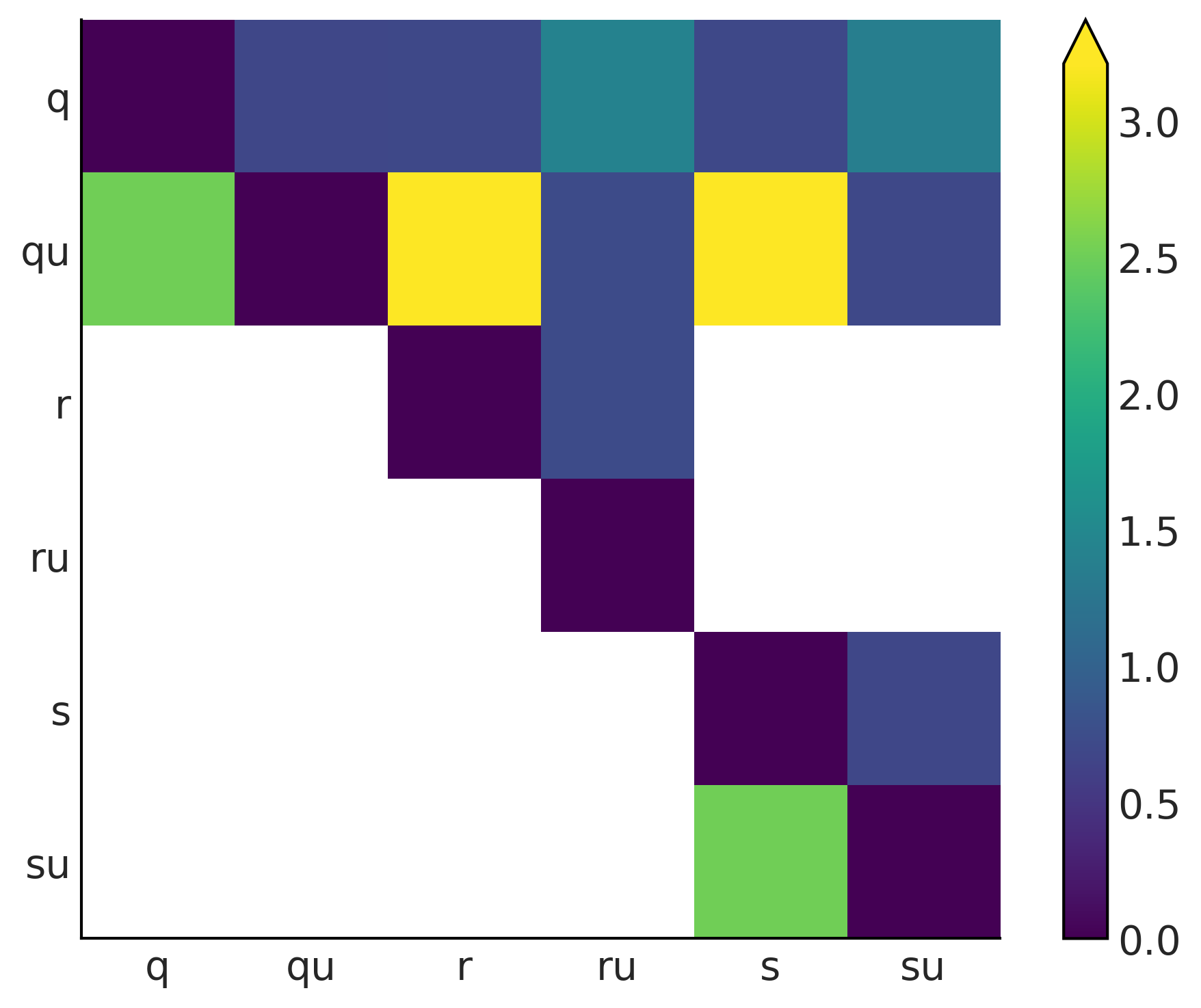
dists = [q_pmf, qu_pmf, r_pmf, ru_pmf, s_pmf, su_pmf]
names = ["q", "qu", "r", "ru", "s", "su"]

fig, ax = plt.subplots()
KL_matrix = np.zeros((6, 6))
for i, dist_i in enumerate(dists):
    for j, dist_j in enumerate(dists):
        KL_matrix[i, j] = stats.entropy(dist_i, dist_j)

ax.set_xticks(np.arange(len(names)))
ax.set_yticks(np.arange(len(names)))
ax.set_xticklabels(names)
ax.set_yticklabels(names)
plt.set_cmap("viridis")
cmap = plt.cm.get_cmap()
cmap.set_bad('w', 0.3)
im = ax.imshow(KL_matrix)
fig.colorbar(im, extend="max");

plt.savefig("img/chp11/KL_heatmap.png")

/var/folders/7p/srk5qjp563l5f9mrjtp44bh800jqsw/T/ipykernel_29663/3750536694.py:16: MatplotlibDeprecationWarning: You are modifying the state of a globally registered colormap. This has been deprecated since 3.3 and in 3.6, you will not be able to modify a registered colormap in-place. To remove this warning, you can make a copy of the colormap first. cmap = mpl.cm.get_cmap("viridis").copy()
  cmap.set_bad('w', 0.3)

def beta_binom(prior, y):
    """
    Compute the marginal-log-likelihood for a beta-binomial model,
    analytically.

    prior : tuple
        tuple of alpha and beta parameter for the prior (beta distribution)
    y : array
        array with "1" and "0" corresponding to the success and fails respectively
    """
    α, β = prior
    success = np.sum(y)
    trials = len(y)
    return np.log(binom(trials, success)) + betaln(α + success, β+trials-success) - betaln(α, β)

def beta_binom_harmonic(prior, y, s=10000):
    """
    Compute the marginal-log-likelihood for a beta-binomial model,
    using the harmonic mean estimator.

    prior : tuple
        tuple of alpha and beta parameter for the prior (beta distribution)
    y : array
        array with "1" and "0" corresponding to the success and fails respectively
    s : int
        number of samples from the posterior
    """
    α, β = prior
    success = np.sum(y)
    trials = len(y)
    posterior_samples = stats.beta(α + success, β+trials-success).rvs(s)
    log_likelihood = stats.binom.logpmf(success, trials, posterior_samples)
    return 1/np.mean(1/log_likelihood)

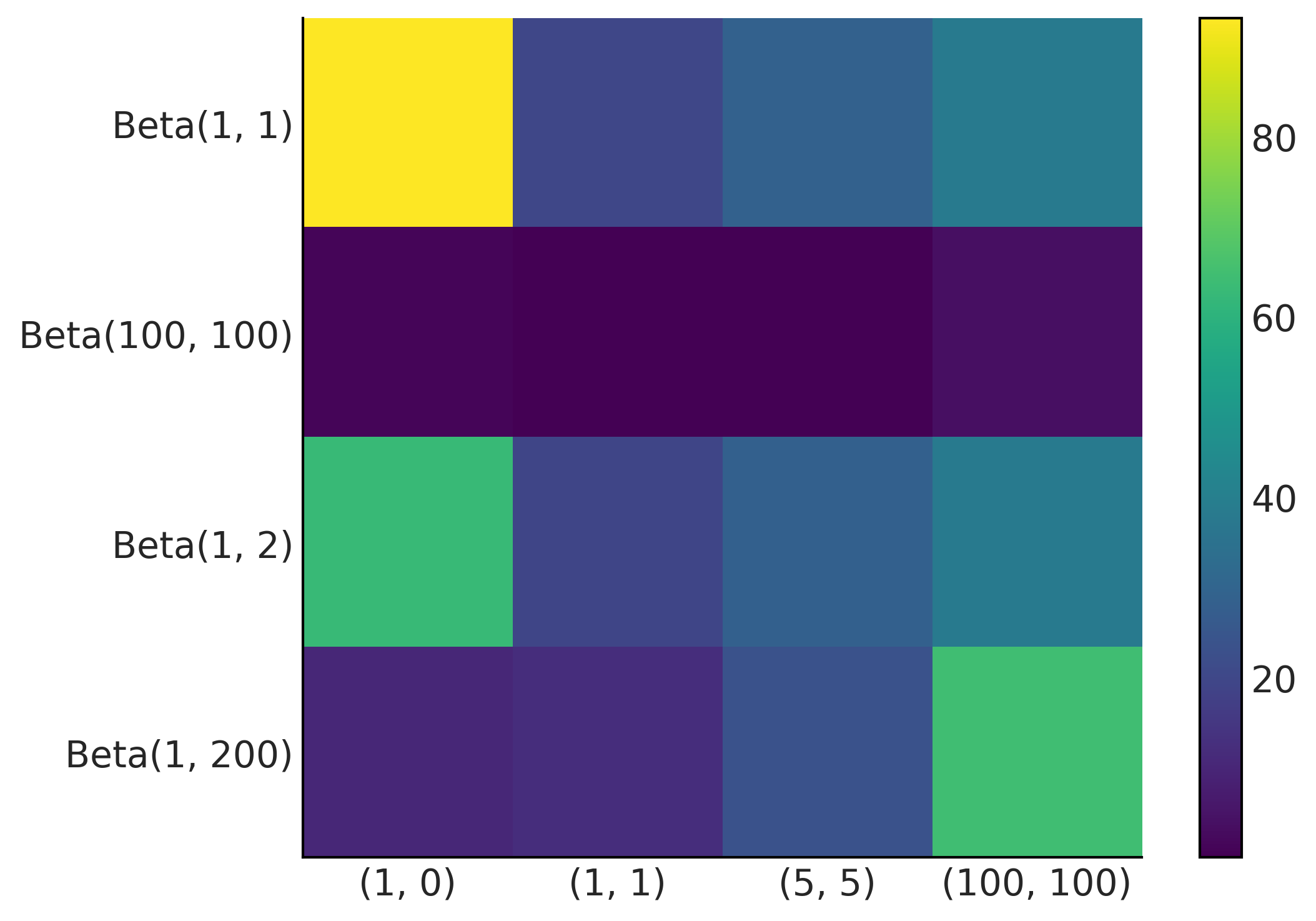
data = [np.repeat([1, 0], rep)
        for rep in ((1, 0), (1, 1), (5, 5), (100, 100))]
priors = ((1, 1), (100, 100), (1, 2), (1, 200))

x_names = [repr((sum(x), len(x)-sum(x))) for x in data]
y_names = ["Beta" + repr(x) for x in priors]

fig, ax = plt.subplots()
error_matrix = np.zeros((len(priors), len(data)))
for i, prior in enumerate(priors):
    for j, y in enumerate(data):
        error_matrix[i, j] = 100 * \
            (1 - (beta_binom_harmonic(prior, y) / beta_binom(prior, y)))
im = ax.imshow(error_matrix, cmap='viridis')
ax.set_xticks(np.arange(len(x_names)))
ax.set_yticks(np.arange(len(y_names)))
ax.set_xticklabels(x_names)
ax.set_yticklabels(y_names)
fig.colorbar(im)
plt.savefig("img/chp11/harmonic_mean_heatmap.png")

def normal_harmonic(sd_0, sd_1, y, s=10000):
    post_tau = 1/sd_0**2 + 1/sd_1**2
    posterior_samples = stats.norm(loc=(y/sd_1**2)/post_tau, scale=(1/post_tau)**0.5).rvs((s, len(x)))
    log_likelihood = stats.norm.logpdf(loc=x, scale=sd_1, x=posterior_samples).sum(1)
    return 1/np.mean(1/log_likelihood)

σ_0 = 1
σ_1 = 1
y = np.array([0])
stats.norm.logpdf(loc=0, scale=(σ_0**2+σ_1**2)**0.5, x=y).sum()

-1.2655121234846454

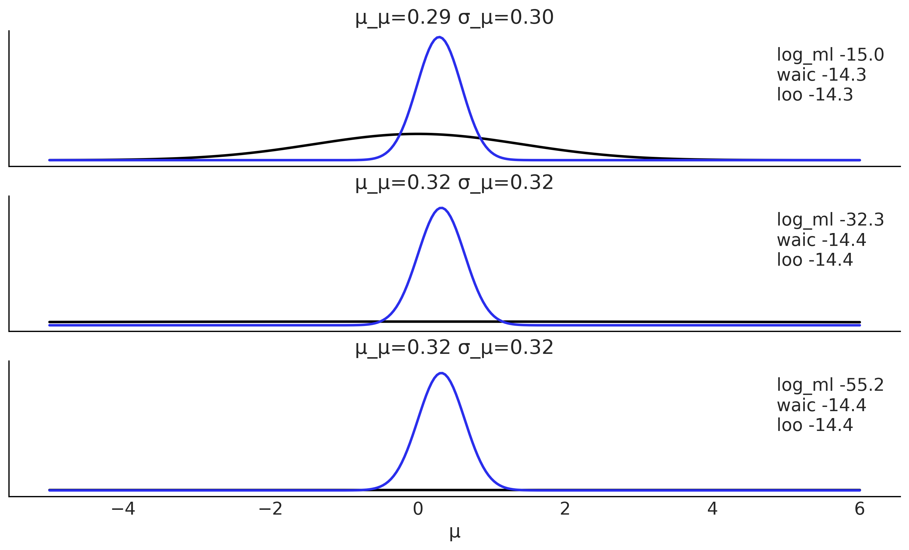
def posterior_ml_ic_normal(σ_0=1, σ_1=1, y=[1]):
    n = len(y)
    var_μ = 1/((1/σ_0**2) + (n/σ_1**2))
    μ = var_μ * np.sum(y)/σ_1**2
    σ_μ = var_μ**0.5

    posterior = stats.norm(loc=μ, scale=σ_μ)
    samples = posterior.rvs(size=(2, 1000))
    log_likelihood = stats.norm(loc=samples[:, :, None], scale=σ_1).logpdf(y)
    idata = az.from_dict(log_likelihood={'o': log_likelihood})

    log_ml = stats.norm.logpdf(loc=0, scale=(σ_0**2+σ_1**2)**0.5, x=y).sum()
    
    x = np.linspace(-5, 6, 300)
    density = posterior.pdf(x)
    
    return μ, σ_μ, x, density, log_ml, az.waic(idata).waic, az.loo(idata, reff=1).loo

y = np.array([ 0.65225338, -0.06122589,  0.27745188,  1.38026371, -0.72751008,
              -1.10323829,  2.07122286, -0.52652711,  0.51528113,  0.71297661])

_, ax = plt.subplots(3, figsize=(10, 6), sharex=True, sharey=True,
                     constrained_layout=True)

for i, σ_0 in enumerate((1, 10, 100)):
    μ_μ, σ_μ, x, density, log_ml, waic, loo = posterior_ml_ic_normal(σ_0, σ_1, y)
    ax[i].plot(x, stats.norm(loc=0, scale=(σ_0**2+σ_1**2)**0.5).pdf(x), lw=2)
    ax[i].plot(x, density, lw=2, color='C4')
    ax[i].plot(0, label=f'log_ml {log_ml:.1f}\nwaic {waic:.1f}\nloo {loo:.1f}\n', alpha=0)
    ax[i].set_title(f'μ_μ={μ_μ:.2f} σ_μ={σ_μ:.2f}')
    ax[i].legend()
ax[2].set_yticks([])

ax[2].set_xlabel("μ")

plt.savefig("img/chp11/ml_waic_loo.png")

σ_0 = 1
σ_1 = 1
y = np.array([0])
stats.norm.logpdf(loc=0, scale=(σ_0**2 + σ_1**2)**0.5, x=y).sum()

-1.2655121234846454

N = 10000
x, y = np.random.uniform(-1, 1, size=(2, N))
inside = (x**2 + y**2) <= 1
pi = inside.sum()*4/N
error = abs((pi - np.pi) / pi) * 100

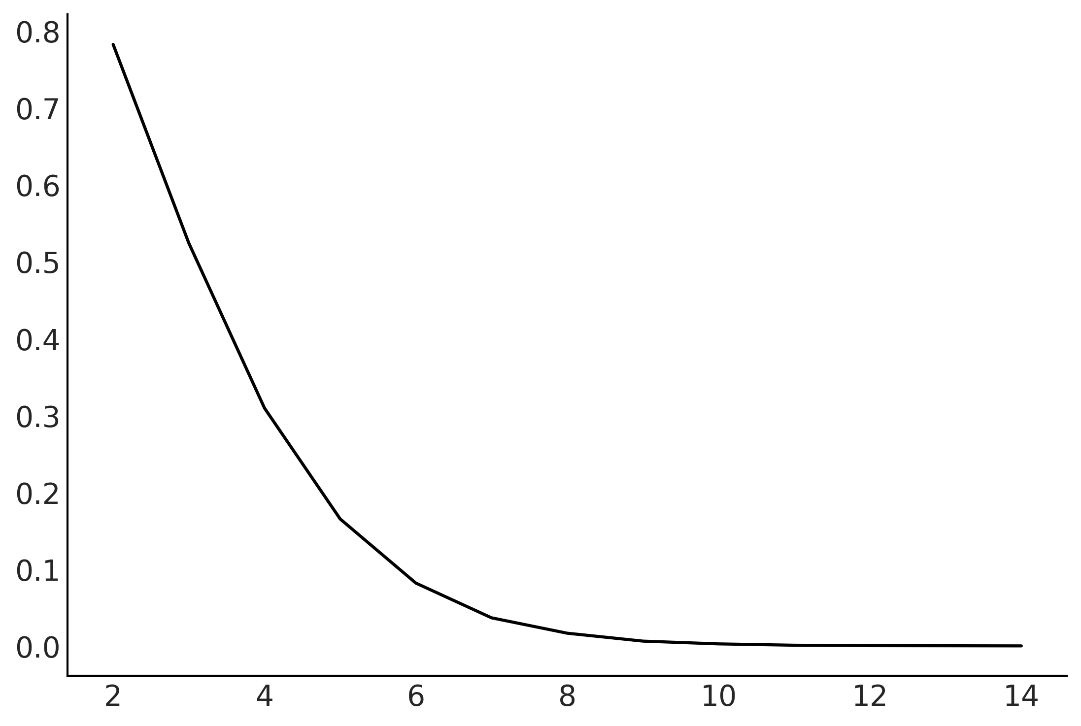
total = 100000

dims = []
prop = []
for d in range(2, 15):
    x = np.random.random(size=(d, total))
    inside = ((x * x).sum(axis=0) < 1).sum()
    dims.append(d)
    prop.append(inside / total)
    
plt.plot(dims, prop);

def posterior_grid(ngrid=10, α=1, β=1, heads=6, trials=9):
    grid = np.linspace(0, 1, ngrid)
    prior = stats.beta(α, β).pdf(grid)
    likelihood = stats.binom.pmf(heads, trials, grid)
    posterior = likelihood * prior
    posterior /= posterior.sum()
    return posterior

Variational Inference

See https://blog.tensorflow.org/2021/02/variational-inference-with-joint-distributions-in-tensorflow-probability.html for a more extended examples

az.style.use("arviz-colors")

import tensorflow as tf
import tensorflow_probability as tfp

tfd = tfp.distributions

# An arbitrary density function as target
target_logprob = lambda x, y: -(1.-x)**2 - 1.5*(y - x**2)**2

# Set up two different surrogate posterior distribution
event_shape = [(), ()]  # theta is 2 scalar
mean_field_surrogate_posterior = tfp.experimental.vi.build_affine_surrogate_posterior(
    event_shape=event_shape, operators="diag")
full_rank_surrogate_posterior = tfp.experimental.vi.build_affine_surrogate_posterior(
    event_shape=event_shape, operators="tril")

# Optimization
losses = []
posterior_samples = []
for approx in [mean_field_surrogate_posterior, full_rank_surrogate_posterior]:
    loss = tfp.vi.fit_surrogate_posterior(
        target_logprob, approx, num_steps=200, optimizer=tf.optimizers.Adam(0.1),
        sample_size=5)
    losses.append(loss)
    # The approx is a tfp distribution, we can sample from it after training
    posterior_samples.append(approx.sample(10000))

WARNING:tensorflow:From /opt/miniconda3/envs/bmcp/lib/python3.9/site-packages/tensorflow/python/ops/linalg/linear_operator_block_diag.py:238: LinearOperator.graph_parents (from tensorflow.python.ops.linalg.linear_operator) is deprecated and will be removed in a future version.
Instructions for updating:
Do not call `graph_parents`.

plt.plot(np.asarray(losses).T)
plt.legend(['mean-field', 'full-rank']);

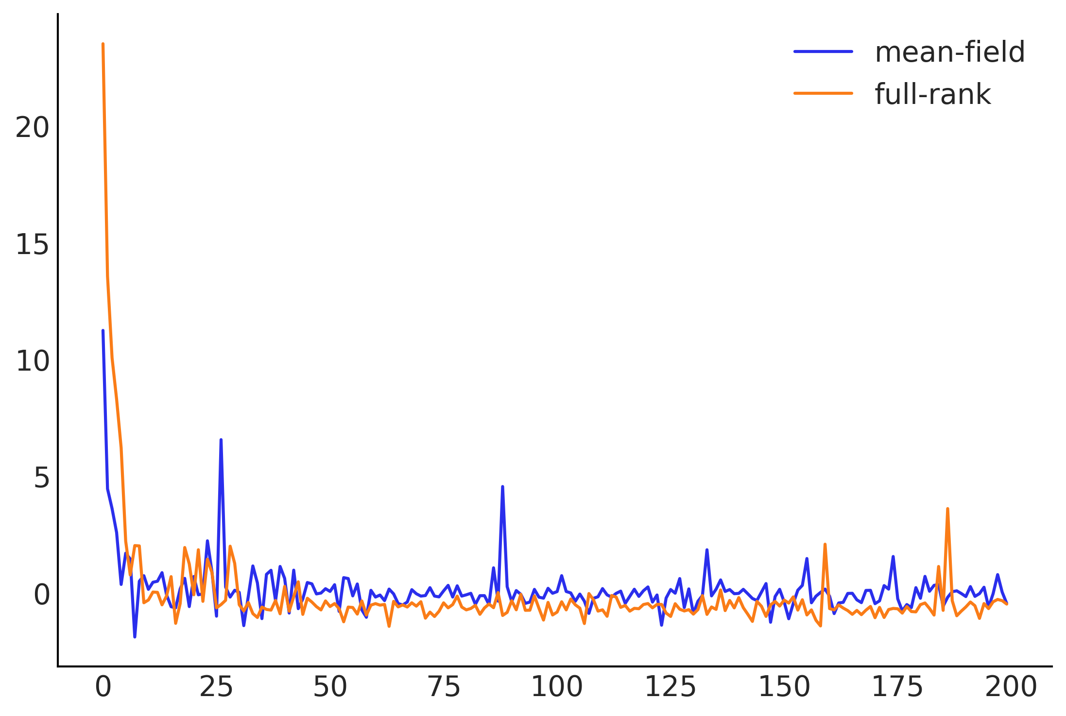
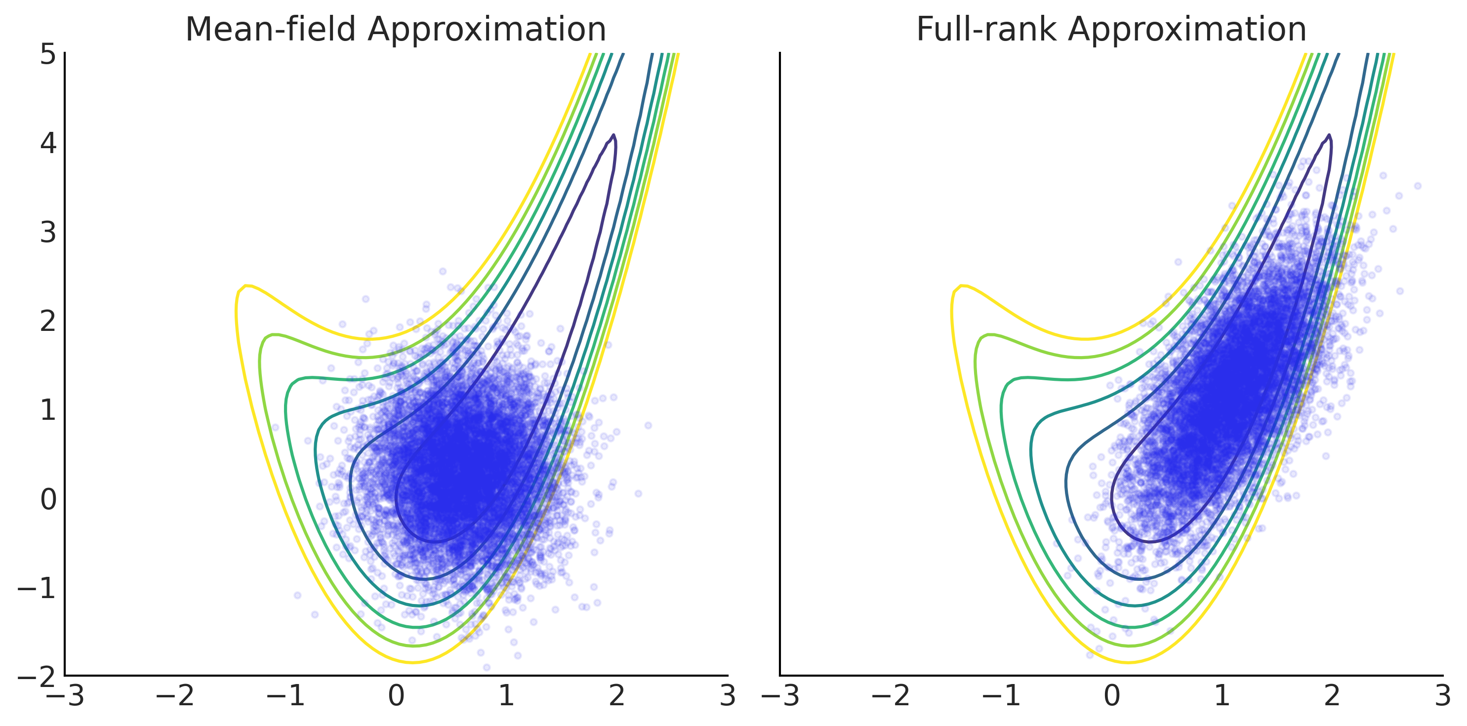
Figure 11.33

grid = np.meshgrid(np.linspace(-3, 3, 100), np.linspace(-2, 5, 100))
Z = - target_logprob(*grid)

_, axes = plt.subplots(1, 2, figsize=(10, 5), sharex=True, sharey=True)
for ax, approx, name in zip(
    axes,
    [mean_field_surrogate_posterior, full_rank_surrogate_posterior],
    ["Mean-field Approximation", "Full-rank Approximation"]):
    ax.contour(*grid, Z, levels=np.arange(7))
    ax.plot(*approx.sample(10000), ".", alpha=.1)
    ax.set_title(name)
plt.tight_layout();

plt.savefig("img/chp11/vi_in_tfp.png")

/var/folders/7p/srk5qjp563l5f9mrjtp44bh800jqsw/T/ipykernel_13440/2635745829.py:12: UserWarning: This figure was using constrained_layout, but that is incompatible with subplots_adjust and/or tight_layout; disabling constrained_layout.
  plt.tight_layout();

VI Deep dive

tfb = tfp.bijectors

event_shape = [(), ()]
full_rank_surrogate_posterior = tfp.experimental.vi.build_affine_surrogate_posterior(
    event_shape=event_shape, operators="tril")

# mean_field_surrogate_posterior = tfp.experimental.vi.build_affine_surrogate_posterior(
#     event_shape=event_shape, operators="diag")
mean_field_surrogate_posterior = tfd.JointDistributionSequential([
    tfd.Normal(tf.Variable(0.), tfp.util.TransformedVariable(1., bijector=tfb.Exp())),
    tfd.Normal(tf.Variable(0.), tfp.util.TransformedVariable(1., bijector=tfb.Exp())),
])

# Density estimation with MADE.
made = tfb.AutoregressiveNetwork(params=2, hidden_units=[10, 10])
flow_surrogate_posterior = tfd.TransformedDistribution(
    distribution=tfd.Sample(tfd.Normal(loc=0., scale=1.), sample_shape=[2]),
    bijector=tfb.Chain([
        tfb.JointMap([tfb.Reshape([]), tfb.Reshape([])]),
        tfb.Split([1, 1]),
        tfb.MaskedAutoregressiveFlow(made)
    ]))
# Create a Masked Autoregressive Flow bijector.
# prior = tfd.JointDistributionSequential([tfd.Normal(0., 1.), tfd.Normal(0., 1.)])
# maf = tfb.MaskedAutoregressiveFlow(shift_and_log_scale_fn=net)
# flow_surrogate_posterior = tfp.experimental.vi.build_split_flow_surrogate_posterior(
#     event_shape=prior.event_shape_tensor(), trainable_bijector=maf)

# Optimization
losses = []
posterior_samples = []
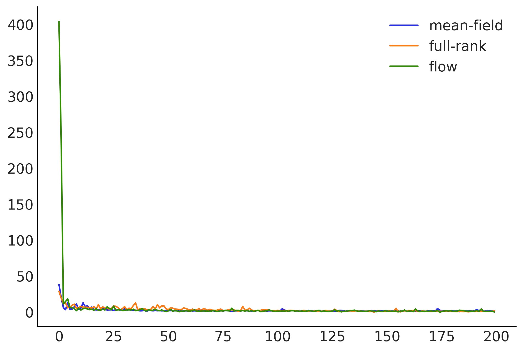
for approx in [mean_field_surrogate_posterior, full_rank_surrogate_posterior, flow_surrogate_posterior]:
    loss = tfp.vi.fit_surrogate_posterior(
        target_logprob, approx, num_steps=200, optimizer=tf.optimizers.Adam(0.1),
        sample_size=5)
    losses.append(loss)
    # The approx is a tfp distribution, we can sample from it after training
    posterior_samples.append(approx.sample(10000))

plt.plot(np.asarray(losses).T)
plt.legend(['mean-field', 'full-rank', 'flow']);

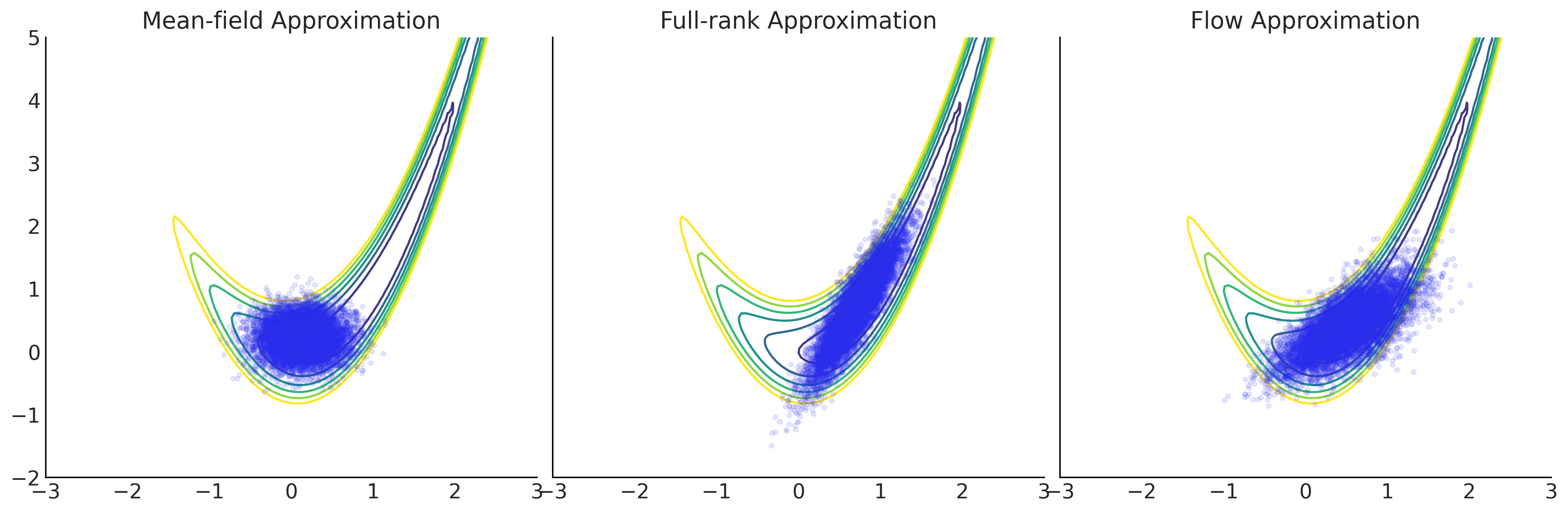
grid = np.meshgrid(np.linspace(-3, 3, 100), np.linspace(-2, 5, 100))
Z = - target_logprob(*grid)

_, axes = plt.subplots(1, 3, figsize=(15, 5), sharex=True, sharey=True)
for ax, approx, name in zip(
    axes,
    [mean_field_surrogate_posterior, full_rank_surrogate_posterior, flow_surrogate_posterior],
    ["Mean-field Approximation", "Full-rank Approximation", "Flow Approximation"]):
    ax.contour(*grid, Z, levels=np.arange(7))
    ax.plot(*approx.sample(10000), ".", alpha=.1)
    ax.set_title(name)
plt.tight_layout();

/var/folders/7p/srk5qjp563l5f9mrjtp44bh800jqsw/T/ipykernel_13440/1954138361.py:12: UserWarning: This figure was using constrained_layout, but that is incompatible with subplots_adjust and/or tight_layout; disabling constrained_layout.
  plt.tight_layout();