Probabilistic Programming Languages

10. Probabilistic Programming Languages#

In Chapter 1 Section Bayesian Modeling, we used cars as analogy to understand applied Bayesian concepts. We will revisit this analogy but this time to understand Probabilistic Programming Languages. If we treat a car as a system, their purpose is to move people or cargo to a chosen destination with wheels connected to a power source. This whole system is presented to users with an interface, typically a steering wheel and pedals. Like all physical objects cars have to obey the laws of physics, but within those bounds human designers have a multitude of components to choose from. Cars can have big engines, or small tires, 1 seat or 8 seats. The end result however, is informed by the specific purpose. Some cars are designed to go fast with a single person around a racetrack, such as Formula 1 cars. Others are designed for family life like carrying families and groceries home from the store. No matter what the purpose, someone needs to pick the components, for the right car, for the right purpose.

The story of Probabilistic Programming Languages (PPL) is similar. The purpose of PPLs is help Bayesian practitioners build generative models to solve problem at hand, for example, perform inference of a Bayesian model through estimating the posterior distribution with MCMC. The power source for computational Bayesians is, well, a computer which are bound by computer science fundamentals. Within those bounds however, PPL designers can choose different components and interfaces, with the specifics being determined by anticipated user need and preference. In this chapter we will focus our discussion on what the components of PPLs are, and different design choices that can be made within those components. This knowledge will help you as Bayesian practitioner when you need to pick a PPL when starting a project or debug that arises during your statistical workflow. This understanding ultimately will lead to better experience for you, the modern Bayesian practitioner.

10.1. A Systems Engineering Perspective of a PPL#

Wikipedia defines systems engineering as “an interdisciplinary field of engineering and engineering management that focuses on how to design, integrate, and manage complex systems over their life cycles”. PPLs are by this definition a complex system. PPLs span across computational backends, algorithms, and base languages. As the definition also states the integration of components is a key part of systems engineering, which is true of PPLs as well. A choice of computational backend can have an effect on the interface, or the choice of base language can limit the available inference algorithms. In some PPLs the user can make component selections themselves. For example, Stan users can choose their base language between R, Python, or the command line interface among others, whereas PyMC3 users cannot change base languages, they must use Python.

In addition to the PPL itself there is the consideration of the organization and manner in which it will be used. A PhD student using a PPL in a research lab has different needs than an engineer working in a corporation. This is also relevant to the lifecycle of a PPL. Researchers may only need a model once or twice in a short period to write a paper, whereas an engineer in a corporation may maintain and run the model over the course of years.

In a PPL the two necessary components are: an application programming interface for the user to define the model [1], and algorithms to performs inference and manage the computation. Other components exist but largely to improve the system in some fashion, such as computational speed or ease of use. Regardless of the choice components, when a system is designed well the day to day user need not be aware of the complexity, just as most drivers are able to use cars without understanding the details of each part. In the ideal case a PPL the user should just feel as though things work just the way they want them. This is the challenge PPL designers must meet.

In the remaining of the chapter, we will give some overview of some general components of a PPL, with examples of design choice from different PPLs. We are not aiming to provide an exhaustive descriptions of all PPLs [2], and we are also not trying to convince you to develop a PPL [3]. Rather, by understanding the implementation consideration, we hope that you will gain a better understanding of how to write more performative Bayesian models, and to diagnose computation bottlenecks and errors when they occur.

10.1.1. Example: Rainier#

Consider the development of Rainier [4], a PPL written in Scala developed at Stripe. Stripe is a payments processing company that handles finances for many thousands of partner business. In Stripe, they need to estimate the distribution of risk associated with each partnered business, ideally with a PPL that is able to support many parallel inferences (one per each business partner) and easy to deploy in Stripe’s compute cluster. As Stripe’s compute clusters included a Java run time environment, they choose Scala as it can be compiled to Java bytecode. Rainier. In this case PyMC3 and Stan were considered as well, but due to either the restriction of Python use (PyMC3), or the requirement for a C++ compiler (Stan), creating a PPL for their particular use case was the best choice.

Most users will not need to develop their own PPL but we present this case study to highlight how considerations of both the environment in which you are using the code, and the functionality of the available PPLs can help inform a decision for a smoother experience as a computational Bayesian.

10.2. Posterior Computation#

Inference is defined as a conclusion reached on the basis of evidence and reasoning and the posterior computational methodology is the engine that gets us to the conclusion. The posterior computation method can largely be thought of as two parts, the computation algorithm, and the software and hardware that makes the calculation, often referred to as the computational backend. When either designing or selecting a PPL, the available posterior computation methods ends up being a key decision that informs many factors of the workflow, from the speed of inference, hardware needed, complexity of PPL, and breadth of applicability. There are numerous algorithms to compute the posterior [5], from exact computations when using conjugate models, to numerical approximations like grid search to Hamiltonian Monte Carlo (HMC), to model approximation like Laplace approximation and variational inference (covered in more detail in Section Variational Inference). When selecting an inference algorithms both the PPL designer and the user need to make a series of choices. For the PPL designer the algorithms have different levels of implementation complexity. For example, conjugate methods are quite easy to implement, as there exists analytical formulas that can be written in a couple lines of code, whereas MCMC samplers are more complex, typically requiring a PPL designer to write much more code than an analytical solution. Another tradeoff in computational complexity, conjugate methods do not require much computation power and can return a posterior in sub millisecond on all modern hardware, even a cell phone. By comparison, HMC is slow and require a system that can compute gradients, such as the one we will present in Section Getting the Gradient. This limits HMC computation to relatively powerful computers, sometimes with specialized hardware.

The user faces a similar dilemma, more advanced posterior computation methods are more general and require less mathematical expertise, but require more knowledge to assess and ensure correct fit. We have seen this throughout this book, where visual and numerical diagnostics are necessary to ensure our MCMC samplers have converged to an estimate of the posterior. Conjugate models do not need any convergence diagnostics due to the fact they calculate the posterior exactly, every time if the right mathematics are used.

For all these reasons there is no universal recommendation for an inference algorithm that suits every situation. At time of writing MCMC methods, especially adaptive Dynamic Hamiltonian Monte Carlo, are the most flexible, but not useful in all situations. As a user it is worthwhile understanding the availability and tradeoffs of each algorithm to be able to make an assessment for each situation.

10.2.1. Getting the Gradient#

An incredibly useful piece of information in computational mathematics is the gradient. Also known as the slope, or the derivative for one dimensional functions, it indicates how fast a function output value is changing at any point in its domain. By utilizing the gradient many algorithms are developed to more efficiently achieve their goal. With inference algorithms we have seen this difference when comparing the Metropolis Hasting algorithm, which does not need a gradient when sampling, to Hamiltonian Monte Carlo, which does use the gradient and usually returns high quality samples faster [6].

Just as Markov chain Monte Carlo was originally developed in the sub field of statistical mechanics before computational Bayesians adopted it, most of the gradient evaluation libraries were originally developed as part of “Deep Learning” libraries mostly intended for backpropagation computation to train Neural Networks. These include Theano, TensorFlow and PyTorch. Bayesians however, learned to use them as computational backends for Bayesian Inference. An example of computational gradient evaluation using JAX [116], a dedicated autograd library, shown in Code Block jax_grad_small. In this Code Block the gradient of \(x^2\) is computed at a value of \(4\). We can solve this analytically with the rule \(rx^{r-1}\), and we can then calculate \(2*4=8\). However, with autograd libraries users do not need to think about closed form solutions. All that is needed is an expression of the function itself and the computer can automatically calculate the gradient, as implied by “auto” in autograd.

Listing 10.1 jax_grad_small#

from jax import grad

simple_grad = grad(lambda x: x**2)
print(simple_grad(4.0))

8.0

Methods such us Adaptive Dynamic Hamiltonian Monte Carlo or Variational Inference use gradients to estimate posterior distributions. Being able to obtain gradient easily becomes even more important when we realize that in posterior computation the gradient typically gets computed thousands of times. We show one such calculation in Code Block jax_model_grad using JAX for a small “hand built” model.

Listing 10.2 jax_model_grad#

from jax import grad
from jax.scipy.stats import norm

def model(test_point, observed):
    z_pdf = norm.logpdf(test_point, loc=0, scale=5)
    x_pdf = norm.logpdf(observed, loc=test_point, scale=1)
    logpdf = z_pdf + x_pdf
    return logpdf

model_grad = grad(model)

observed, test_point = 5.0, 2.5 
logp_val = model(test_point, observed)
grad = model_grad(test_point, observed)
print(f"log_p_val: {logp_val}")
print(f"grad: {grad}")

log_p_val: -6.697315216064453
grad: 2.4000000953674316

For comparison we can make the same calculation using a PyMC3 model and computing the gradient using Theano in Code Block pymc3_model_grad.

Listing 10.3 pymc3_model_grad#

with pm.Model() as model:
    z = pm.Normal("z", 0., 5.)
    x = pm.Normal("x", mu=z, sd=1., observed=observed)

func = model.logp_dlogp_function()
func.set_extra_values({})
print(func(np.array([test_point])))

[array(-6.69731498), array([2.4])]

From the output we can see the PyMC3 model returns the same logp and gradient as the JAX model.

10.2.2. Example: Near Real Time Inference#

As a hypothetical example consider a statistician at a credit card company that is concerned with detecting credit card fraud quickly so it can disable cards before the thief can make more transactions. A secondary system classifies transactions as fraudulent or legitimate but the company wants to ensure it does not block cards with a low number of events and wants to be able to set priors for different customers to control the sensitivity. It is decided that the users accounts will be disabled when mean of the posterior distribution is above a probability threshold of 50%. In this near real time scenario inference needs to be performed in less than a second so fraudulent activity can be detected before the transaction clears. The statistician recognizes that this can be analytically expressed using a conjugate model which she then writes in Equation (10.1), where the \(\alpha\) and \(\beta\) parameters, representing the prior of fraud and non-fraud transactions directly. As transactions are observed they are used fairly directly compute the posterior parameters.

(10.1)#\[ \begin{align}\begin{aligned}\begin{split}\begin{split} \alpha_\text{post} &= \alpha_\text{prior} + \texttt{fraud_observations} \\ \beta_\text{post} &= \beta_\text{prior} + \texttt{non_fraud_observations} \\ % p(\theta) &= \text{Beta}(fraud\_prior, non\_fraud\_prior) \\ p(\theta \mid y) &= \text{Beta}(\alpha_\text{post}, \beta_\text{post}) \\ \mathop{\mathbb{E}}[p(\theta \mid y)] &= \frac{\alpha_\text{post}}{\alpha_\text{post} + \beta_\text{post}}\end{split}\\\end{split}\end{aligned}\end{align} \]

She can then fairly trivially express these calculations in Python as shown in Code Block fraud_detector. No external libraries needed either, making this function quite easy to deploy.

Listing 10.4 fraud_detector#

def fraud_detector(fraud_observations, non_fraud_observations, fraud_prior=8, non_fraud_prior=6):
    """Conjugate Beta Binomial model for fraud detection"""
    expectation = (fraud_prior + fraud_observations) / (
        fraud_prior + fraud_observations + non_fraud_prior + non_fraud_observations)
    
    if expectation > .5:
        return {"suspend_card":True}

%timeit fraud_detector(2, 0)

152 ns ± 0.969 ns per loop (mean ± std. dev. of 7 runs, 100 loops each)

To meet the sensitivity and probability computation time requirements of less than one second a conjugate prior is selected, and the model posterior is calculated in Code Block fraud_detector. The calculations took about 152 ns, in contrast an MCMC sampler will take around 2 seconds on the same machine which is over 6 orders of magnitude. It is unlikely that any MCMC sampler would meet the time requirement needed from this system, making a conjugate prior the clear choice.

Hardware and Sampling Speed

From a hardware perspective, there are three ways to increase MCMC sampling speed. The first is typically the clock speed of the processing unit, often measured in hertz, or Gigahertz for modern computers. This is the speed at which the instructions are executed, so generally speaking a 4 Gigahertz computer can execute twice as many instructions in a second than a 2 Gigahertz computer. In MCMC sampling the clock speed will correlate with the number of samples that can be taken in a timespan for a single chain. The other is parallelization across multiple cores in a processing unit. In MCMC sampling each chains can be sampled in parallel on computers with multiple cores. This coincidentally is convenient as many convergence metrics use multiple chains. On a modern desktop computer anywhere from 2 to 16 cores are typically available. The last method is specialized hardware such as the Graphics Processing Units (GPUs) and Tensor Processing Units (TPUs). If paired with the correct software and algorithms these are able to both sample each chain more quickly, but also sample more chains in parallel.

10.3. Application Programming Interfaces#

Application Programming Interfaces (API) “define interactions between multiple software intermediaries”. In the Bayesian case the most narrow definition is the interactions between the user and the method to compute the posterior. At its most broad it can include multiple steps in the Bayesian workflow, such as specifying a random variable with a distribution, linking different random variables to create the model, prior and posterior predictive checks, plotting, or any task. The API is typically first part, and sometimes the only part, a PPL practitioner interactions with and typically is where the practitioner spends the most amount of time. API design is both a science and an art and designers must balance multiple concerns.

On the science side PPLs must be able to interface with a computer and provide the necessary elements to control the computation methods. Many PPLs are defined with base languages and typically need to follow the fixed computational constraints of the base language as well as the computational backend. In Section Example: Near Real Time Inference, only a 4 parameters and one line of code were needed to obtain an exact result. Contrast this with MCMC examples that had various inputs such as number of draws, acceptance rate, number of tuning steps and more. The complexity of MCMC, while mostly hidden, still surfaced additional complexity in the API.

So many APIs, so many interfaces

In a modern Bayesian workflow there is not just the PPL API but APIs of all the supporting packages in the workflow. In this book we have also used the Numpy, Matplotlib, Scipy, Pandas and ArviZ APIs across examples, not to mention the Python API itself. In the Python ecosystem. These choices of packages, and the APIs they bring, are also subject to personal choice. A practitioner may choose to use Bokeh as a replacement to Matplotlib for plotting, or xarray in addition to pandas, and in doing so the user will need to learn those APIs as well.

In addition to just APIs there are many code writing interfaces to write Bayesian models, or just code in general. Code can be written in the text editors, notebook, Integrated Development Environments (IDEs), or the command line directly.

The use of these tools, both the supporting packages and the coding interface, is not mutually exclusive. For someone new to computational statistics this can be a lot to take in. When starting out we suggest using a simple text editor and a few supporting packages to allow for your focus to be on the code and model, before moving onto more complex interfaces such as notebooks or Integrated Development Environments. We provide more guidance regarding this topic in Section Text Editor vs Integrated Development Environment vs Notebook.

On the art side API is the interface for human users. This interface is one of the most important parts of the PPL. Some users tend to have strong, albeit subjective views, about design choices. Users want the simplest, most flexible, readable, and easy to write API, objectives which, for the poor PPL designer, are both ill defined and opposed with each other. One choice a PPL designer can make is to mirror style and functionality of the base language. For example, there is a notion of “Pythonic” programs which are follow in a certain style [7]. This notion of pythonic API is what informs the PyMC3 API, the goal is to explicitly have users feel like they are writing their models in Python. In contrast Stan models are written in a domain specific language informed by other PPLs such as BUGS [117] and languages such as C++ [118]. The Stan language includes notable API primitives such as curly braces and uses a block syntax as shown in Code Block code_stan. Writing a Stan model distinctly does not feel like writing Python, but this is not a knock against the API. It is just a different choice from a design standpoint and a different experience for the user.

10.3.1. Example: Stan and Slicstan#

Depending on the use case, user might prefer different level of abstraction in terms model specification, independent of any other PPL component. Stan and Slicstan using from Gorinova etal {cite:p}`Gorinova_2019] which is specifically dedicated to studying and proposing Stan APIs. In Code Block code_stan we show the, original, Stan model syntax. In the Stan syntax various pieces of a Bayesian model are indicated by blocks declarations. These names correspond with the various sections of the workflow, such as specifying the model and parameters, data transformations, prior and posterior predictive sampling, with corresponding names such as parameters, model, transformed parameters, and generated quantities.

Listing 10.5 code_stan#

parameters {
    real y_std;
    real x_std;
}
transformed parameters {
    real y = 3 * y_std;
    real x = exp(y/2) * x_std;
}
model {
    y_std ~ normal(0, 1);
    x_std ~ normal(0, 1);
}

An alternative syntax for Stan models is Slicstan [119], the same model of which is shown in Code Block slicstan. Slicstan provides a compositional interface to Stan, letting users define functions which can be named and reused, and does away with the block syntax. These features mean Slicstan programs can be expressed in less code than standard Stan models. While not always the most important metric less code means less code that the Bayesian modeler needs to write, and less code that a model reviewer needs to read. Also, like Python, composable functions allow the user to define an idea once and reuse it many times, such as my_normal in the Slicstan snippet.

Listing 10.6 slicstan#

real my_normal(real m, real s) {
real std ~ normal(0, 1);
    return s * std + m;
}
real y = my_normal(0, 3);
real x = my_normal(0, exp(y/2));

For the original Stan syntax, it has the benefit of familiarity (for those who already use it) and documentation. The familiarity may come from Stan’s choice to model itself after BUGS ensuring that users who have prior experience with that language, will be comfortable transitioning to the Stan syntax. It also is familiar for people who have been using Stan for numerous years. Since it was released 2012, there have now been multiple years for users to get familiar with the language, publish examples, and write models. For new users the block model forces organization so when writing a Stan program they will end up being more consistent.

Note both Stan and Slicstan use the same codebase under the API layer the difference in API is solely for the benefit of the user. In this case which API is “better” is a choice for each user. We should note this case study is only a shallow discussion of the Stan API. For full details we suggest reading the full paper, which formalizes both sets of syntax and shows the level of detail goes into API design.

10.3.2. Example: PyMC3 and PyMC4#

Our second API is a case study of an API design change that was required because of a computational backend change, in this case from Theano in PyMC3 to TensorFlow in PyMC4 a PPL that was initially intended to replace PyMC3 [120]. In the design of PyMC4 the designers of the language desired to keep the syntax as close as possible to the PyMC3 syntax. While the inference algorithms remained the same, the fundamental way in which TensorFlow and Python works meant the PyMC4 API forced into a particular design due to the change in computational backend. Consider the Eight Schools model [27] implemented in PyMC3 syntax in Code Block pymc3_schools and the now, defunct [8] PyMC4 syntax in Code Block pymc4_schools.

Listing 10.7 pymc3_schools#

with pm.Model() as eight_schools_pymc3:
    mu = pm.Normal("mu", 0, 5)
    tau = pm.HalfCauchy("tau", 5)
    theta = pm.Normal("theta", mu=mu, sigma=tau, shape=8)
    obs = pm.Normal("obs", mu=theta, sigma=sigma, observed=y)

Listing 10.8 pymc4_schools#

@pm.model
def eight_schools_pymc4():
    mu = yield pm.Normal("mu", 1, 5)
    tau = yield pm.HalfNormal("tau", 5)
    theta = yield pm.Normal("theta", loc=mu, scale=sigma, batch_stack=8)

    obs = yield pm4.Normal("obs", loc=theta, scale=sigma, observed=y)
    return obs

The differences in PyMC4 is the decorator @pm.model, the declaration of a Python function, the use of generators indicated by yield, and differing argument names. You may have noticed that the yield is the same that you have seen in the TensorFlow Probability code. In both PPLs yield statement was a necessary part of the API due to the choice coroutine. These APIs changes were not desired however, as users would have to learn a new syntax, all existing PyMC3 code would have to be rewritten to use PyMC4, and all existing PyMC3 documentation would become obsolete. This is an example where the API is informed not by user preference, but by the choice computational backend used to calculate the posterior. In the end the feedback from users to keep the PyMC3 API unchanged was one of the reasons to terminate PyMC4 development.

10.4. PPL Driven Transformations#

In this book we saw many mathematical transformations that allowed us to define a variety of models, easily and with great flexibility such as GLMs. Or we saw transformations that allowed us to make results more interpretable such as centering. In this section we will specifically discuss transformations that are driven more specifically by PPL. They are sometimes a bit implicit and we will discuss two examples in this section.

10.4.1. Log Probabilities#

One of the most common transformations is the log probability transform. To understand why let us go through an example where we calculate an arbitrary likelihood. Assume we observe two independent outcomes \(y_0\) and \(y_1\), their joint probability is:

(10.2)#\[p(y_0, y_1 \mid \boldsymbol{\theta}) = p(y_0 \mid \boldsymbol{\theta})p(y_1 \mid \boldsymbol{\theta}) \]

To give a specific situation let us say we observed the value 2 twice and we decide to use a Normal distribution as a likelihood in our model. We can specify our model by expanding Equation (10.2) into:.

(10.3)#\[\mathcal{N}(2, 2 \mid \mu=0,\sigma=1) = \mathcal{N}(2 \mid 0,1)\mathcal{N}(2 \mid 0,1) \]

Being computational statisticians we can now calculate this value with a little bit of code.

Listing 10.9 two_observed#

observed = np.repeat(2, 2)
pdf = stats.norm(0, 1).pdf(observed)
np.prod(pdf, axis=0)

0.0029150244650281948

With two observations we get 20 decimals of precision for joint probability density in Code Block two_observed with no issues, but now let us assume we see a total of 1000 observations, all of the same value of 2. We can repeat our calculation in Code Block thousand_observed. This time however, we have an issue, Python reports a joint probability density of 0.0, which cannot be true.

Listing 10.10 thousand_observed#

observed = np.repeat(2, 1000)
pdf = stats.norm(0, 1).pdf(observed)
np.prod(pdf, axis=0)

0.0

What we are seeing is an example of floating point precision error in computers. Due to the fundamental way computers store numbers in memory and evaluate calculations, only a limited amount of precision is possible. In Python this error in precision is often hidden from the user [9], although in certain cases the user is exposed to the lack of precision, as shown in Code Block imperfect_subtract

Listing 10.11 imperfect_subtract#

1.2 - 1

0.19999999999999996

With relatively “large” numbers the small error in the far decimal place matter little. However, in Bayesian modeling we often are working with very small float point numbers, and even worse we multiply them together many times making them smaller yet. To mitigate this problem PPLs perform a log transformation of probability often abbreviated to logp. Thus expression (10.2) turns into:

(10.4)#\[\log (p(y_0, y_1 \mid \boldsymbol{\theta})) = \log (p(y_0 \mid \boldsymbol{\theta}))+ \log (p(y_1 \mid \boldsymbol{\theta})) \]

This has two effects, it makes small numbers relatively large, and due to the product rule of logarithms, changes the multiplication into a sum. Using the same example but performing the calculation in log space, we see a more numerically stable result in Code Block log_transform.

Listing 10.12 log_transform#

logpdf = stats.norm(0, 1).logpdf(observed)

# Compute individual logpdf two ways for one observation, as well as total
np.log(pdf[0]), logpdf[0], logpdf.sum()

(-2.9189385332046727, -2.9189385332046727, -2918.9385332046736)

10.4.2. Random Variables and Distributions Transformations#

Random variables that distributed as a bounded distributions, like the Uniform distribution that is specified with a fixed interval \([a, b]\), present a challenge for gradient evaluation and samplers based on them. Sudden changes in geometry make it difficult to sample the distribution at the neighborhood of those sudden changes. Imagine rolling a ball down a set of stairs or a cliff, rather than a smooth surface. It is easier to estimate the trajectory of the ball over a smooth surface rather than the discontinuous surface. Thus, another useful set of transformations in PPLs [10] are transformations that turn bounded random variables, such as those distributed as Uniform, Beta, Halfnormal, etc, into unbounded random variables that span entire real line from (\(-\infty\), \(\infty\)). These transformations however, need to be done with care as we must now correct for the volume changes in our transformed distributions. To do so we need to compute the Jacobians of the transformation and accumulate the calculated log probabilities, explained in further detail in Section Transformations.

PPLs usually transform bounded random variables into unbounded random variables and perform inference in the unbounded space, and then transform back the values to the original bounded space, all can happen without user input. Thus users do not need to interact with these transformations if they do not want to. For a concrete example both the forward and backward transform for the Uniform random variable are shown in Equation (10.5) and computed in Code Block interval_transform. In this transformation the lower and upper bound \(a\) and \(b\) are mapped to \(-\infty\) and \(\infty\) respectively, and the values in between are “stretched” to values in between accordingly.

(10.5)#\[\begin{split}\begin{split} x_t =& \log (x - a) - \log(b-x)\\ x =& a + \frac{1}{1 + e^{-x_t}} (b-a) \end{split}\end{split}\]

Listing 10.13 interval_transform#

lower, upper = -1, 2
domain = np.linspace(lower, upper, 5)
transform = np.log(domain - lower) - np.log(upper - domain)
print(f"Original domain: {domain}")
print(f"Transformed domain: {transform}")

Original domain:[-1.   -0.25  0.5   1.25  2.  ]
Transformed domain: [-inf -1.09861229, 0., 1.09861229, inf]

The automatic transform can be seen by adding a Uniform random variable to a PyMC3 model and inspecting the variable and the underlying distribution in the model object, as shown in Code Block uniform_transform.

Listing 10.14 uniform_transform#

with pm.Model() as model:
    x = pm.Uniform("x", -1., 2.)

model.vars

([x_interval__ ~ TransformedDistribution])

Seeing this transform we can also then query the model to check the transformed logp values in Code Block uniform_transform_logp. Note how with the transformed distribution we can sample outside of the interval \((-1, 2)\) (the boundaries of the un-transformed Uniform) and still obtain a finite logp value. Also note the logp returned from the logp_nojac method, and how the value is the same for the values of -2 and 1, and how when we call logp the Jacobian adjustment is made automatically.

Listing 10.15 uniform_transform_logp#

print(model.logp({"x_interval__":-2}),
      model.logp_nojac({"x_interval__":-2}))
print(model.logp({"x_interval__":1}),
      model.logp_nojac({"x_interval__":1}))

-2.2538560220859454 -1.0986122886681098
-1.6265233750364456 -1.0986122886681098

Log transformation of the probabilities and unbounding of random variables are transformations that PPLs usually apply without most users knowing, but they both have a practical effect on the performance and usability of the PPL across a wide variety of models.

There are other more explicit transformations users can perform directly on the distribution itself to construct new distribution. User can then create random variables distributed as these new distributions in a model. For example, the bijectors module [2] in TFP can be used to transform a base distribution into more complicated distributions. Code Block bijector_lognormal demonstrates how to construct a \(LogNormal(0, 1)\) distribution by transforming the base distribution \(\mathcal{N}(0, 1)\) [11]. This expressive API design even allows users to define complicated transformation using trainable bijectors (e.g., a neural network [121]) like tfb.MaskedAutoregressiveFlow.

Listing 10.16 bijector_lognormal#

tfb = tfp.bijectors

lognormal0 = tfd.LogNormal(0., 1.)
lognormal1 = tfd.TransformedDistribution(tfd.Normal(0., 1.), tfb.Exp())
x = lognormal0.sample(100)

np.testing.assert_array_equal(lognormal0.log_prob(x), lognormal1.log_prob(x))

Whether explicitly used, or implicitly applied, we note that these transformations of random variables and distributions are not a strictly required components of PPLs, but certainly are included in nearly every modern PPL in some fashion. For example, they can be incredibly helpful in getting good inference results efficiently, as shown in the next example.

10.4.3. Example: Sampling Comparison between Bounded and Unbounded Random Variables#

Here we create a small example to demonstrate the differences between sampling from transformed and un-transformed random variable. Data is simulated from a Normal distribution with a very small standard deviation and model is specified in Code Block case_study_transform.

Listing 10.17 case_study_transform#

y_observed = stats.norm(0, .01).rvs(20)

with pm.Model() as model_transform:
    sd = pm.HalfNormal("sd", 5)
    y = pm.Normal("y", mu=0, sigma=sd, observed=y_observed)
    trace_transform = pm.sample(chains=1, draws=100000)

print(model_transform.vars)
print(f"Diverging: {trace_transform.get_sampler_stats('diverging').sum()}")

[sd_log__ ~ TransformedDistribution()]
Diverging: 0

We can inspect free variables and after sampling we can count the number of divergences. From the code output from Code Block case_study_transform we can verify the bounded HalfNormal sd variable has been transformed, and in subsequent sampling there are no divergences.

For a counterexample, let us specify the same model in Code Block case_study_no_transform but in this case the HalfNormal prior distribution explicitly was not transformed. This is reflected both in the model API, as well as when inspecting the models free variables. Subsequent sampling sampling reports 423 divergences.

Listing 10.18 case_study_no_transform#

with pm.Model() as model_no_transform:
    sd = pm.HalfNormal("sd", 5, transform=None)
    y = pm.Normal("y", mu=0, sigma=sd, observed=y_observed)
    trace_no_transform = pm.sample(chains=1, draws=100000)

print(model_no_transform.vars)
print(f"Diverging: {trace_no_transform.get_sampler_stats('diverging').sum()}")

[sd ~ HalfNormal(sigma=10.0)]
Diverging: 423

In the absence of automatic transforms the user would need to spend some time assessing why the divergences are occurring, and either know that a transformation is needed from prior experience or come to this conclusion through debugging and research, all efforts that take time away from building the model and performing inference.

10.5. Operation Graphs and Automatic Reparameterization#

One manipulation that some PPLs perform is reparameterizing models, by first creating an operation graph and then subsequently optimizing that graph. To illustrate what this means let us define a computation:

(10.6)#\[\begin{split}\begin{split} x=3 \\ y=1 \\ x*(y/x) + 0 \end{split}\end{split}\]

Humans, with basic algebra knowledge, will quickly see that the \(x\) terms cancel leaving the addition \(y+0\), which has no effect, leading to an answer of 1. We can also perform this calculation in pure Python and get the same answer which is great, but what is not great is the wasted computation. Pure Python, and libraries like numpy, just see these operations as computational steps and will faithfully perform each step of the stated equation, first dividing \(y\) by \(x\), then multiplying that result by \(x\), then adding 0.

In contrast libraries like Theano work differently. They first construct a symbolic representation of the computation as shown in Code Block unoptimized_symbolic_algebra.

Listing 10.19 unoptimized_symbolic_algebra#

x = theano.tensor.vector("x")
y = theano.tensor.vector("y")
out = x*(y/x) + 0
theano.printing.debugprint(out)

Elemwise{add,no_inplace} [id A] ''   
 |Elemwise{mul,no_inplace} [id B] ''   
 | |x [id C]
 | |Elemwise{true_div,no_inplace} [id D] ''   
 |   |y [id E]
 |   |x [id C]
 |InplaceDimShuffle{x} [id F] ''   
   |TensorConstant{0} [id G]

What is Aesara?

As you have seen Theano is the workhorse of PyMC3 models in terms of graph representation, gradient calculation, and much more. However, Theano was deprecated in 2017 by the original authors. Since then PyMC developers have been maintaining Theano to support of PyMC3. In 2020 the PyMC developers decided to move from maintaining Theano to improving it. In doing so the PyMC developers forked Theano and named the fork Aesara [12]. With a focused effort led by Brandon Willard the legacy portions of the code base have been drastically modernized. Additionally Aesara includes expanded functionality particularly for Bayesian use cases. These include adding new backends (JAX and Numba) for accelerated numerical computation and better support modern compute hardware such GPU and TPU. With greater control and coordination over more of the PPL components between the PyMC3 and Aesara the PyMC developers are looking to continuously foster a better PPL experience for developers, statisticians, and users.

In the output of Code Block unoptimized_symbolic_algebra, working inside out, we see on Line 4 the first operation is the division of \(x\) and \(y\), then the multiplication \(x\), then finally the addition of 0 represented in a computation graph. This same graph is shown visually in Fig. 10.1. At this point no actual numeric calculations have taken place, but a sequence of operations, albeit an unoptimized one, has been generated.

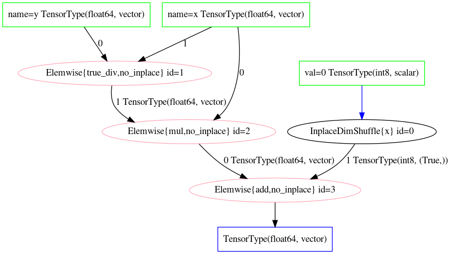
../_images/symbolic_graph_unopt.png — Fig. 10.1 Unoptimized Theano operation graph of Equation (10.6) as declared in Code Block unoptimized_symbolic_algebra.#

We can now optimize this graph using Theano, by passing this computation graph to theano.function in Code Block optimized_symbolic_algebra. In the output nearly all the operations have disappeared, as Theano has recognized that both multiplication and division of \(x\) cancels out, and that the addition of \(0\) has no effect on the final outcome. The optimized operation graph is shown in Fig. 10.2.

Listing 10.20 optimized_symbolic_algebra#

fgraph = theano.function([x,y], [out])
theano.printing.debugprint(fgraph)

DeepCopyOp [id A] 'y'   0
 |y [id B]

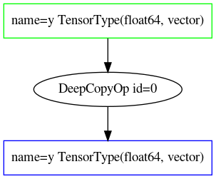
../_images/symbolic_graph_opt.png — Fig. 10.2 Optimized Theano operation graph of Equation (10.6) after optimization in optimized_symbolic_algebra.#

Theano can then calculate the answer when the optimized function is called with the numerical inputs as shown in Code Block optimized_symbolic_algebra_calc.

Listing 10.21 optimized_symbolic_algebra_calc#

fgraph([1],[3])

[array([3.])]

To perform the algebraic simplication, your computer did not become sentient and rederive the rules of algebra from scratch. Theano is able to perform these optimizations thanks to a code optimizer [13] that inspects the operation graph stated through the Theano API by a user, scans the graph for algebraic patterns, and simplifies computation and give users the desired result.

Bayesian models are just a special case of both mathematics and computation. In Bayesian computation typically desired output is the logp of the model. Before optimization the first step is a symbolic representation of the operations graph, an example of which is shown in Code Block aesara_debug where a one line PyMC3 model is turned into multi line computation graph at the operation level.

Listing 10.22 aesara_debug#

with pm.Model() as model_normal:
    x = pm.Normal("x", 0., 1.)

theano.printing.debugprint(aesara_normal.logpt)

Sum{acc_dtype=float64} [id A] '__logp'   
 |MakeVector{dtype='float64'} [id B] ''   
   |Sum{acc_dtype=float64} [id C] ''   
     |Sum{acc_dtype=float64} [id D] '__logp_x'   
       |Elemwise{switch,no_inplace} [id E] ''   
         |Elemwise{mul,no_inplace} [id F] ''   
         | |TensorConstant{1} [id G]
         | |Elemwise{mul,no_inplace} [id H] ''   
         |   |TensorConstant{1} [id I]
         |   |Elemwise{gt,no_inplace} [id J] ''   
         |     |TensorConstant{1.0} [id K]
         |     |TensorConstant{0} [id L]
         |Elemwise{true_div,no_inplace} [id M] ''   
         | |Elemwise{add,no_inplace} [id N] ''   
         | | |Elemwise{mul,no_inplace} [id O] ''   
         | | | |Elemwise{neg,no_inplace} [id P] ''   
         | | | | |TensorConstant{1.0} [id Q]
         | | | |Elemwise{pow,no_inplace} [id R] ''   
         | | |   |Elemwise{sub,no_inplace} [id S] ''   
         | | |   | |x ~ Normal(mu=0.0, sigma=1.0) [id T]
         | | |   | |TensorConstant{0.0} [id U]
         | | |   |TensorConstant{2} [id V]
         | | |Elemwise{log,no_inplace} [id W] ''   
         | |   |Elemwise{true_div,no_inplace} [id X] ''   
         | |     |Elemwise{true_div,no_inplace} [id Y] ''   
         | |     | |TensorConstant{1.0} [id Q]
         | |     | |TensorConstant{3.141592653589793} [id Z]
         | |     |TensorConstant{2.0} [id BA]
         | |TensorConstant{2.0} [id BB]
         |TensorConstant{-inf} [id BC]

Just like algebraic optimization this graph can then be optimized in ways that benefit the Bayesian user [122]. Recall the discussion in Section Posterior Geometry Matters, certain models benefit from non-centered parameterizations, as this helps eliminate challenging geometry such as Neal’s funnel. Without automatic optimization the user must be aware of the geometrical challenge to the sampler and make the adjust themselves. In the future, libraries such as symbolic-pymc [14] will be able to make this reparameterization automatic, just as we say the automatic transformation of log probability and bounded distributions above. With this upcoming tool PPL users can further focus on the model and let the PPL “worry” about the computational optimizations.

10.6. Effect handling#

Effect handlers [123] are an abstraction in programming languages that gives different interpretations, or side effects, to the standard behavior of statements in a program. A common example is exception handling in Python with try and except. When some specific error is raised in the code block under try statement, we can perform different processing in the except block and resume computation. For Bayesian models there are two primary effects we want the random variable to have, draw a value (sample) from its distribution, or condition the value to some user input. Other use cases of effect handlers are transforming bounded random variables and automatic reparameterization as we mentioned above.

Effect handlers are not a required component of PPLs but rather a design choice that strongly influences the API and the “feel” of using the PPL. Harkening back to our car analogy this is similar to a power steering system in a car. It is not required, it is usually hidden from the driver under the hood but it definitely changes the driving experience. As effect handlers are typically “hidden” they are more easily explained through example rather than theory.

10.6.1. Example: Effect Handling in TFP and Numpyro#

In the rest of this section we will see how effect handling works in TensorFlow Probability and NumPyro. Briefly NumPyro is another PPL based on Jax. Specifically, we will compare the high level API between tfd.JointDistributionCoroutine and model written with NumPyro primitives, which both represent Bayesian model with a Python function in a similar way. Also, we will be using the JAX substrate of TFP, so that both API share the same base language and numerical computation backend. Again consider the model in Equation (10.7), in Code Block tfp_vs_numpyro we import the libraries and write the model:

Listing 10.23 tfp_vs_numpyro#

import jax
import numpyro
from tensorflow_probability.substrates import jax as tfp_jax

tfp_dist = tfp_jax.distributions
numpyro_dist = numpyro.distributions

root = tfp_dist.JointDistributionCoroutine.Root
def tfp_model():
    x = yield root(tfp_dist.Normal(loc=1.0, scale=2.0, name="x"))
    z = yield root(tfp_dist.HalfNormal(scale=1., name="z"))
    y = yield tfp_dist.Normal(loc=x, scale=z, name="y")
    
def numpyro_model():
    x = numpyro.sample("x", numpyro_dist.Normal(loc=1.0, scale=2.0))
    z = numpyro.sample("z", numpyro_dist.HalfNormal(scale=1.0))
    y = numpyro.sample("y", numpyro_dist.Normal(loc=x, scale=z))

From a glance, tfp_model and numpyro_model looks similar, both are Python functions with no input argument and return statement (note NumPyro model can have inputs and return statements), both need to indicate which statement should be considered as random variable (TFP with yield, NumPyro with numpyro.sample primitives). Moreover, the default behavior of both tfp_model and numpyro_model is ambiguous, they do not really do anything [15] until you give it specific instruction. For example, in Code Block tfp_vs_numpyro_prior_sample we draw prior samples from both models, and evaluate the log probability on the same prior samples (that returned by the TFP model).

Listing 10.24 tfp_vs_numpyro_prior_sample#

sample_key = jax.random.PRNGKey(52346)

# Draw samples
jd = tfp_dist.JointDistributionCoroutine(tfp_model)
tfp_sample = jd.sample(1, seed=sample_key)

predictive = numpyro.infer.Predictive(numpyro_model, num_samples=1)
numpyro_sample = predictive(sample_key)

# Evaluate log prob
log_likelihood_tfp = jd.log_prob(tfp_sample)
log_likelihood_numpyro = numpyro.infer.util.log_density(
    numpyro_model, [], {},
    # Samples returning from JointDistributionCoroutine is a
    # Namedtuple like Python object, we convert it to a dictionary
    # so that numpyro can recognize it.
    params=tfp_sample._asdict())

# Validate that we get the same log prob
np.testing.assert_allclose(log_likelihood_tfp, log_likelihood_numpyro[0])

We can also condition some random variable to user input value in our model, for example, in Code Block tfp_vs_numpyro_condition we condition z = .01 and then sample from the model.

Listing 10.25 tfp_vs_numpyro_condition#

# Condition z to .01 in TFP and sample
jd.sample(z=.01, seed=sample_key)

# Condition z to .01 in NumPyro and sample
predictive = numpyro.infer.Predictive(
    numpyro_model, num_samples=1, params={"z": np.asarray(.01)})
predictive(sample_key)

From user perspective effect handling mostly happens behind the scenes when high level APIs are used. In TFP a tfd.JointDistribution encapsulate the effect handlers inside of a single object, and change the behavior of a function within that object when the input arguments are different. For NumPyro the effect handling is a bit more explicit and flexible. A set of effect handlers are implemented in numpyro.handlers, which powers the high level APIs we just used to generate prior samples and compute model log probability. This is shown again in Code Block tfp_vs_numpyro_condition_distribution, where we conditioned random variable \(z = .01\), draw a sample from \(x\), and construct conditional distribution \(p(y \mid x, z)\) and sample from it.

Listing 10.26 tfp_vs_numpyro_condition_distribution#

# Conditioned z to .01 in TFP and construct conditional distributions
dist, value = jd.sample_distributions(z=.01, seed=sample_key)
assert dist.y.loc == value.x
assert dist.y.scale == value.z

# Conditioned z to .01 in NumPyro and construct conditional distributions
model = numpyro.handlers.substitute(numpyro_model, data={"z": .01})
with numpyro.handlers.seed(rng_seed=sample_key):
    # Under the seed context, the default behavior of a NumPyro model is the
    # same as in Pyro: drawing prior sample.
    model_trace = numpyro.handlers.trace(numpyro_model).get_trace()
assert model_trace["y"]["fn"].loc == model_trace["x"]["value"]
assert model_trace["y"]["fn"].scale == model_trace["z"]["value"]

The Python assertion in Code Block tfp_vs_numpyro_condition_distribution is to validate that the conditional distribution is indeed correct. Compare to the jd.sample_distributions(.) call, You could see the explicit effect handling in NumPyro with numpyro.handlers.substitute that returns a conditioned model, numpyro.handlers.seed to set the random seed (a JAX requirement for drawing random samples), and numpyro.handlers.trace to trace the function execution. More information of the effect handling in NumPyro and Pyro could be found in their official documentation [16].

10.7. Base Language, Code Ecosystem, Modularity and Everything Else#

When serious car enthusiasts pick a car, the availability of different components that can be mixed and match can be an informative factor in which car is ultimately purchased. These owners may choose to make aesthetic changes to fit their preference such as a new hood for a different look, or they may choose to perform an engine swap, which substantially changes the performance of the vehicle. Regardless most car owners would prefer to have more choices and flexibility in how they can modify their vehicle then less, even if they do not choose to modify their vehicle at all.

In this same way PPL users are not only concerned about the PPL itself, but also what related code bases and packages exist in that particular ecosystem, as well as the modularity of the PPL itself. In this book we have used Python as the base language, and PyMC3 and TensorFlow Probability as our PPLs. With them however, we have also used Matplotlib for plotting, NumPy for numerical operations, Pandas and xarray for data manipulation, and ArviZ for exploratory analysis of Bayesian models. Colloquially these are all part of the PyData stack. However, there are other base languages such as R with their own ecosystem of packages. This ecosystem has similar set of tools under the tidyverse moniker, as well as specific Bayesian packages aptly named loo, posterior, bayesplot among others. Luckily Stan users are able to change base languages relatively easily, as the model is defined in the Stan language and there is a choice of interfaces available such as pystan, rstan, cmdstan and others. PyMC3 users are relegated to Python. However, with Theano there is modularity in the computational backend that can be used, from the Theano native backend, to the newer JAX backend. Along with all the above there is a laundry list of other points that matter, non-uniformly, to PPL users including.

Ease of development in production environments
Ease of installation in development environment
Developer speed
Computational speed
Availability of papers, blog posts, lectures
Documentation
Useful error messages
The community
What colleagues recommend
Upcoming features

Just having choices is not enough however, to use a PPL a user must be able to install and understand how to use them. The availability of work that references the PPL tends to indicate how widely accepted it is and provide confidence that it is indeed useful. Users are not keen to invest time into a PPL that will no longer be maintained. And ultimately as humans, even data informed Bayesian users, the recommendation of a respected colleagues and other presence of a large user base, are all influential factors in evaluating PPL, as much as the technical capabilities in many circumstances.

10.8. Designing a PPL#

In this section we will switch our perspective from a PPL overview as a user and to one of a PPL designer. Now that we identified the big components let us design a hypothetical PPL to see how components fit together and also how they sometimes do not fit as easily as you would hope! The choices we will make are for illustrative purposes but frame how the system comes together, and also how a PPL designer thinks when putting together a PPL.

First we choose a base language with a numerical computing backend. Since this book focuses on Python let us use NumPy. Ideally, we also have a set of commonly used mathematical functions implemented for us already. For example, the central piece for implementing a PPL is a set of (log)probability mass or density function, and some pseudo random number generators. Luckily, those are readily available via scipy.stats. Let us put these together in Code Block scipy_stats with a simple demonstration of drawing some samples from a \(\mathcal{N}(1, 2)\) distribution and evaluate their log probability:

Listing 10.27 scipy_stats#

import numpy as np
from scipy import stats

# Draw 2 samples from a Normal(1., 2.) distribution
x = stats.norm.rvs(loc=1.0, scale=2.0, size=2, random_state=1234)
# Evaluate the log probability of the samples 
logp = stats.norm.logpdf(x, loc=1.0, scale=2.0)

where stats.norm is a Python class in the scipy.stats module [17] which contains methods and statistical functions associated with the family of Normal distributions. Alternatively, we can initialize a Normal distribution with fixed parameters as shown in Code Block scipy_stats2.

Listing 10.28 scipy_stats2#

random_variable_x = stats.norm(loc=1.0, scale=2.0)

x = random_variable_x.rvs(size=2, random_state=1234)
logp = random_variable_x.logpdf(x)

Both Code Blocks scipy_stats and scipy_stats2 return exactly the same output x and logp as we also supplied the same random_state. The differences here is that Code Block scipy_stats2 we have a “frozen” random variable [18] random_variable_x that could be considered as the SciPy representation of \(x \sim \mathcal{N}(1, 2)\). Unfortunately, this object does work well when we try to use it naively when writing a full Bayesian models. Consider the model \(x \sim \mathcal{N}(1, 2), y \sim \mathcal{N}(x, 0.1)\). Writing it in Code Block simple_model_not_working_scipy raises an exception because scipy.stats.norm is expecting the input to be a NumPy array [19].

Listing 10.29 simple_model_not_working_scipy#

x = stats.norm(loc=1.0, scale=2.0)
y = stats.norm(loc=x, scale=0.1)
y.rvs()

...
TypeError: unsupported operand type(s) for +: 'float' and 'rv_frozen'

From this it becomes evident how tricky it is to design an API, what seems intuitive for the user may not be possible with the underlying packages, In our case to write a PPL in Python we need to make a series of API design choices and other decision to make Code Block simple_model_not_working_scipy work. Specifically we want:

A representation of random variables that could be used to initialize another random variable;
To be able to condition the random variable on some specific values (e.g., the observed data);
The graphical model, generated by a collection of random variables, to behave in a consistent and predictable way.

Getting Item 1 to work is actually pretty straightforward with a Python class that could be recognized by NumPy as an array. We do this in Code Block scipy_rv0 and use the implementation to specific the model in Equation (10.7).

(10.7)#\[\begin{split}\begin{split} x \sim& \mathcal{N}(1, 2) \\ z \sim& \mathcal{HN}(1) \\ y \sim& \mathcal{N}(x, z) \end{split}\end{split}\]

Listing 10.30 scipy_rv0#

class RandomVariable:
    def __init__(self, distribution):
        self.distribution = distribution

    def __array__(self):
        return np.asarray(self.distribution.rvs())

x = RandomVariable(stats.norm(loc=1.0, scale=2.0))
z = RandomVariable(stats.halfnorm(loc=0., scale=1.))
y = RandomVariable(stats.norm(loc=x, scale=z))

for i in range(5):
    print(np.asarray(y))

7362186279475353
5877468494932253
916129854385227
7421638350544257
074813968631388

A more precise description for the Python class we wrote in Code Block scipy_rv0 is a stochastic array. As you see from the Code Block output, instantiation of this object, like np.asarray(y), always gives us a different array. Adding a method to conditioned the random variable to some value, with a log_prob method, we have in Code Block scipy_rv1 a toy implementation of a more functional RandomVariable:

Listing 10.31 scipy_rv1#

class RandomVariable:
    def __init__(self, distribution, value=None):
        self.distribution = distribution
        self.set_value(value)
    
    def __repr__(self):
        return f"{self.__class__.__name__}(value={self.__array__()})"

    def __array__(self, dtype=None):
        if self.value is None:
            return np.asarray(self.distribution.rvs(), dtype=dtype)
        return self.value

    def set_value(self, value=None):
        self.value = value
    
    def log_prob(self, value=None):
        if value is not None:
            self.set_value(value)
        return self.distribution.logpdf(np.array(self))

x = RandomVariable(stats.norm(loc=1.0, scale=2.0))
z = RandomVariable(stats.halfnorm(loc=0., scale=1.))
y = RandomVariable(stats.norm(loc=x, scale=z))

We can look at the value of y with or without conditioning the value of its dependencies in Code Block scipy_rv1_value, and the output seems to match the expected behavior. In Code Block below note how y is much closer to x if we set z to a small value.

Listing 10.32 scipy_rv1_value#

for i in range(3):
    print(y)

print(f"  Set x=5 and z=0.1")
x.set_value(np.asarray(5))
z.set_value(np.asarray(0.05))
for i in range(3):
    print(y)

print(f"  Reset z")
z.set_value(None)
for i in range(3):
    print(y)

RandomVariable(value=5.044294197842362)
RandomVariable(value=4.907595148778454)
RandomVariable(value=6.374656988711546)
  Set x=5 and z=0.1
RandomVariable(value=4.973898547458924)
RandomVariable(value=4.959593974224869)
RandomVariable(value=5.003811456458226)
  Reset z
RandomVariable(value=6.421473681641824)
RandomVariable(value=4.942894375257069)
RandomVariable(value=4.996621204780431)

Moreover, we can evaluate the unnormalized log probability density of the random variable. For example, in Code Block scipy_rv1_posterior we generate the posterior distribution for x and z when we observe y = 5.0.

Listing 10.33 scipy_rv1_posterior#

# Observed y = 5.
y.set_value(np.array(5.))

posterior_density = lambda xval, zval: x.log_prob(xval) + z.log_prob(zval) + y.log_prob()
posterior_density(np.array(0.), np.array(1.))

-15.881815599614018

We can validate it with an explicit implementation of the posterior density function, as shown in Code Block scipy_posterior:

Listing 10.34 scipy_posterior#

def log_prob(xval, zval, yval=5):
    x_dist = stats.norm(loc=1.0, scale=2.0)
    z_dist = stats.halfnorm(loc=0., scale=1.)
    y_dist = stats.norm(loc=xval, scale=zval)
    return x_dist.logpdf(xval) + z_dist.logpdf(zval) + y_dist.logpdf(yval)

log_prob(0, 1)

-15.881815599614018

At this point, it seems we have fulfilled the requirements of Item 1 and Item 2 , but Item 3 is the most challenging [20]. For example, in a Bayesian workflow we want to draw prior and prior predictive sample from a model. While our RandomVariable draws a random sample according to its prior, when it is not conditioned on some value, it does not record the values of its parents (in a graphical model sense). We need additional graph utilities assign to RandomVariable so that the Python object aware of its parents and children (i.e., its Markov blanket), and propagates the change accordingly if we draw a new sample or conditioned on some specific value [21]. For example, PyMC3 uses Theano to represent the graphical model and keep track of the dependencies (see Section Operation Graphs and Automatic Reparameterization above) and Edward [22] uses TensorFlow v1 [23] to achieve that.

Spectrum of Probabilistic Modelling Libraries

One aspect of PPLs that is worth mentioning is universality. A universal PPL is a PPL that is Turing-complete. Since the PPLs used in this book are an extension of a general-purpose base language, they could all be considered Turing-complete. However, research and implementation dedicated to universal PPLs usually focus on areas slightly different from what we discussed here. For example, an area of focus in a universal PPL is to express dynamic models, where the model contains complex control flow that dependent on random variable [124]. As a result, the number of random variables or the shape of a random variable could change during the execution of a dynamic probabilistic model. A good example of universal PPLs is Anglican [125]. Dynamic models might be valid or possible to write down, but there might not be an efficient and robust method to inference them. In this book, we discuss mainly PPLs focusing on static models (and their inference), with a slight sacrifice and neglect of universality. On the other end of the spectrum of universality, there are great software libraries that focus on some specific probabilistic models and their specialized inference [24], which could be better suited for user’s applications and use cases.

Another approach is to treat model in a more encapsulated way and write the model as a Python function. Code Block scipy_posterior gave an example implementation of the joint log probability density function of the model in Equation (10.7), but for prior samples we need to again rewrite it a bit, shown in Code Block scipy_prior:

Listing 10.35 scipy_prior#

def prior_sample():
    x = stats.norm(loc=1.0, scale=2.0).rvs()
    z = stats.halfnorm(loc=0., scale=1.).rvs()
    y = stats.norm(loc=x, scale=z).rvs()
    return x, z, y

With effect handling and function tracing [25] in Python, we can actually combine log_prob from Code Block scipy_posterior and sample from Code Block scipy_prior into a single Python function the user just need to write once. The PPL will then change the behavior of how the function is executed depending on the context (whether we are trying to obtain prior samples or evaluate the log probability). This approach of writing a Bayesian model as function and apply effect handler has gained significant popularity in recent years with Pyro [126] (and NumPyro [127]), Edward2 [128, 129], and JointDistribution in TensorFlow Probability [29] [26] [27].

10.8.1. Shape Handling in PPLs#

Something that all PPLs must deal with, and subsquently PPL designers must think about, is shapes. One of the common requests for help and frustrations that PPL designers hear from Bayesian modeler and practitioner are about shape errors. They are misspecification of the intended flow of array computation, which can cause issues like broadcasting errors. In this section we will give some examples to highly some subtleties of shape handling in PPLs.

Consider the prior predictive sample function defined in Code Block scipy_prior for the model in Equation (10.7), executing the function draws a single sample from the prior and prior predictive distribution, it is certainly quite inefficient if we want to draw a large among of iid samples from it. Distribution in scipy.stats has a size keyword argument to allow us to draw iid samples easily, with a small modification in Code Block prior_batch we have:

Listing 10.36 prior_batch#

def prior_sample(size):
    x = stats.norm(loc=1.0, scale=2.0).rvs(size=size)
    z = stats.halfnorm(loc=0., scale=1.).rvs(size=size)
    y = stats.norm(loc=x, scale=z).rvs()
    return x, z, y

print([x.shape for x in prior_sample(size=(2))])
print([x.shape for x in prior_sample(size=(2, 3, 5))])

[(2,), (2,), (2,)]
[(2, 3, 5), (2, 3, 5), (2, 3, 5)]

As you can see, the function can handle arbitrary sample shape by adding size keyword argument when calling the random method rvs. Note however, for random variable y, we do not supply the size keyword argument as the sample shape is already implied from its parents.

Consider another example in Code Block prior_lm_batch for a linear regression model, we implemented lm_prior_sample0 to draw one set of prior samples, and lm_prior_sample to draw a batch of prior samples.

Listing 10.37 prior_lm_batch#

n_row, n_feature = 1000, 5
X = np.random.randn(n_row, n_feature)

def lm_prior_sample0():
    intercept = stats.norm(loc=0, scale=10.0).rvs()
    beta = stats.norm(loc=np.zeros(n_feature), scale=10.0).rvs()
    sigma = stats.halfnorm(loc=0., scale=1.).rvs()
    y_hat = X @ beta + intercept
    y = stats.norm(loc=y_hat, scale=sigma).rvs()
    return intercept, beta, sigma, y

def lm_prior_sample(size=10):
    if isinstance(size, int):
        size = (size,)
    else:
        size = tuple(size)
    intercept = stats.norm(loc=0, scale=10.0).rvs(size=size)
    beta = stats.norm(loc=np.zeros(n_feature), scale=10.0).rvs(
        size=size + (n_feature,))
    sigma = stats.halfnorm(loc=0., scale=1.).rvs(size=size)
    y_hat = np.squeeze(X @ beta[..., None]) + intercept[..., None]
    y = stats.norm(loc=y_hat, scale=sigma[..., None]).rvs()
    return intercept, beta, sigma, y

Comparing the two functions above, we see that to make the prior sample function to handle arbitrary sample shape, we need to make a few changes in lm_prior_sample:

Supply size keyword argument to the sample call of root random variables only;
Supply size + (n_feature,) keyword argument to the sample call of beta due to API limitations, which is a length n_feature vector of regression coefficient. We need to additionally make sure size is a tuple in the function so that it could be combined with the original shape of beta;
Shape handling by appending a dimension to beta, intercept, and sigma, and squeezing of the matrix multiplication result so that they are broadcast-able.

As you can see, there is a lot of room for error and flexibility of how you might go about to implementing a “shape-safe” prior sample function. The complexity does not stop here, shape issues also pop up when computing model log probability and during inference (e.g., how non-scalar sampler MCMC kernel parameters broadcast to model parameters). There are convenience function transformations that vectorize your Python function such as numpy.vectorize or jax.vmap in JAX, but they are often not a silver bullet solution to fixing the all issues. For example, it requires additional user input if the vectorization is across multiple axes.

An example of a well defined shape handling logic is the shape semantic in TensorFlow Probability [2] [28], which conceptually partitions a Tensor’s shape into three groups:

Sample shape that describes iid draws from the distribution.
Batch shape that describes independent, not identically distributed draws. Usually it is a set of (different) parameterizations to the same distribution.
Event shape that describes the shape of a single draw (event space) from the distribution. For example, samples from multivariate distributions have non-scalar event shape.

Explicit batch shape is a powerful concept in TFP, which can be considered roughly along the line of independent copy of the same thing that I would like to “parallelly” evaluate over. For example, different chains from a MCMC trace, a batch of observation in mini-batch training, etc. For example, applying the shape semantic to the prior sample function in Code Block prior_lm_batch, we have a beta distributed as a n_feature batch of \(\mathcal{N}(0, 10)\) distribution. Note that while it is fine for the purpose of prior sampling, to be more precise we actually want the Event shape being n_feature instead of the batch shape. In that case the shape is correct for both forward random sampling and inverse log-probability computation. In NumPy it could be done by defining and sampling from a stats.multivariate_normal instead.

When a user defines a TFP distribution, they can inspect the batch shape and the event shape to make sure it is working as intended. It is especially useful when writing a Bayesian model using tfd.JointDistribution. For example, we rewrite the regression model in Code Block prior_lm_batch into Code Block jd_lm_batch using tfd.JointDistributionSequential:

Listing 10.38 jd_lm_batch#

jd = tfd.JointDistributionSequential([
    tfd.Normal(0, 10),
    tfd.Sample(tfd.Normal(0, 10), n_feature),
    tfd.HalfNormal(1),
    lambda sigma, beta, intercept: tfd.Independent(
        tfd.Normal(
            loc=tf.einsum("ij,...j->...i", X, beta) + intercept[..., None],
            scale=sigma[..., None]),
        reinterpreted_batch_ndims=1,
        name="y")
])

print(jd)

n_sample = [3, 2]
for log_prob_part in jd.log_prob_parts(jd.sample(n_sample)):
    assert log_prob_part.shape == n_sample

tfp.distributions.JointDistributionSequential 'JointDistributionSequential' 
batch_shape=[[], [], [], []] 
event_shape=[[], [5], [], [1000]] 
dtype=[float32, float32, float32, float32]

A key thing to look for when ensuring the model is specified correctly is that batch_shape are consistent across arrays. In our example they are since they are all empty. Another helpful way to check that output is a structure of Tensor with the same shape k when calling jd.log_prob_parts(jd.sample(k)) (line 15-17 in Code Block jd_lm_batch). This will make sure the computation of the model log probability (e.g., for posterior inference) is correct. You can find a nice summary and visual demonstration of the shape semantic in TFP in a blog post by Eric J. Ma (Reasoning about Shapes and Probability Distributions) [29].

10.9. Takeaways for the Applied Bayesian Practitioner#

We want to stress to the reader that the goal of this chapter is not to make you a proficient PPL designer but more so an informed PPL user. As a user, particularly if you are just starting out, it can be difficult to understand which PPL to choose and why. When you first learn about a PPL, it is good to keep in mind the basic components we listed in this chapter. For example, what primitives parameterize a distribution, how to evaluate the log-probability of some value, or what primitives define a random variables and how to link different random variables to construct a graphical model (the effect handling) etc.

There are many considerations when picking PPL aside from the PPL itself. Given everything we have discussed in this chapter so far its very easy to get lost trying to optimize over each component to “pick the best one”. Its also very easy for experienced practitioners to argue about why one PPL is better than another ad nauseum. Our advice is to pick the PPL that you feel most comfortable starting with and learn what is needed in your situation from applied experience.

However, over time you will get a sense of what you need from a PPL and more importantly what you do not. We suggest trying out a couple of PPLs, in addition to the ones presented in this book, to get a sense of what will work for you. As a user you have the most to gain from actually using the PPL.

Like Bayesian modeling when you explore the distribution of possibilities the collection of data becomes more informative than any single point. With the knowledge of how PPLs are constructed from this chapter, and personal experience through “taking some for a spin” we hope you will be finding the one that works best for you.

10.10. Exercises#

10E1. Find a PPLs that utilizes another base language other than Python. Determine what differences are between PyMC3 or TFP. Specifically note a difference between the API and the computational backend.

10E2. In this book we primarily use the PyData ecosystem. R is another popular programming language with a similar ecosystem. Find the R equivalents for

Matplotlib
The ArviZ LOO function
Bayesian visualization

10E3. What are other transformations that we have used on data and models throughout this book? What effect did they have? Hint: Refer to Chapter [3]](chap2)

10E4. Draw a block diagram of a PPL[30]. Label each component and explain what it does in your own words. There is no one right answer for this question.

10E5. Explain what batch shape, event shape, and sample shape are in your own words. In particular be sure to detail why its helpful to have each concept in a PPL.

10E6. Find the Eight Schools NumPyro example online. Compare this to the TFP example, in particular noting the difference in primitives and syntax. What is similar? What is different?

10E7. Specify the following computation in Theano

(10.8)#\[\sin(\frac{1}{2}\pi x) + \exp(\log(x)) + \frac{(x-2)^2}{(x^2-4x+4)}\]

Generate the unoptimized computational graph. How many lines are printed. Use the theano.function method to run the optimizer. What is different about the optimized graph? Run a calculation using the optimized Theano function where \(x=1\). What is the output value?

10M8. Create a model with following distributions using PyMC3.

Gamma(alpha=1, beta=1)
Binomial(p=5,12)
TruncatedNormal(mu=2, sd=1, lower=1)

Verify which distributions are automatically transformed from bounded to unbounded distributions. Plot samples from the priors for both the bounded priors and their paired transforms if one exists. What differences can you note?

10H9. BlackJAX is a library of samplers for JAX. Generate a random sample of from \(\mathcal(N)(0,10)\) of size 20. Use the HMC sampler in JAX to recover the parameters of the data generating distribution. The BlackJAX documentation and Section Hamiltonian Monte Carlo will be helpful.

10H10. Implement the linear penguins model defined in Code Block non_centered_regression in NumPyro. After verifying the result are roughly the same as TFP and PyMC3, what differences do you see from the TFP and PyMC3 syntax? What similarities do you see? Be sure not just compare models, but compare the entire workflow.

10H11. We have explained reparameterization in previous chapter, for example, center and non-center parameterization for linear model in Section Posterior Geometry Matters. One of the use case for effect handling is to perform automatic reparameterization [130]. Try to write a effect handler in NumPyro to perform automatic non-centering of a random variable in a model. Hint: NumPyro already provides this functionality with numpyro.handlers.reparam.