3. Linear Models and Probabilistic Programming Languages

With the advent of Probabilistic Programming Languages, modern Bayesian modeling can be as simple as coding a model and “pressing a button”. However, effective model building and analysis usually takes more work. As we progress through this book we will be building many different types of models but in this chapter we will start with the humble linear model. Linear models are a broad class of models where the expected value of a given observation is the linear combination of the associated predictors. A strong understanding of how to fit and interpret linear models is a strong foundation for the models that will follow. This will also help us to consolidate the fundamentals of Bayesian inference (Chapter 1) and exploratory analysis of Bayesian models (Chapter 2) and apply them with different PPLs. This chapter introduces the two PPLs we will use for the majority of this book, PyMC3, which you have briefly seen, as well as TensorFlow Probability (TFP). While we are building models in these two PPLs, focusing on how the same underlying statistical ideas are mapped to implementation in each PPL. We will first fit an intercept only model, that is a model with no covariates, and then we will add extra complexity by adding one or more covariates, and extend to generalized linear models. By the end of this chapter you will be more comfortable with linear models, more familiar with many of the steps in a Bayesian workflow, and more comfortable conducting Bayesian workflows with PyMC3, TFP and ArviZ.

3.1. Comparing Two (or More) Groups

If you are looking for something to compare it is hard to beat penguins. After all, what is not to like about these cute flightless birds? Our first question may be “What is the average mass of each penguin species?”, or may be “How different are those averages?”, or in statistics parlance “What is the dispersion of the average?” Luckily Kristen Gorman also likes studying penguins, so much so that she visited 3 Antarctic islands and collected data about Adelie, Gentoo and Chinstrap species, which is compiled into the Palmer Penguins dataset [28]. The observations consist of physical characteristics of the penguin mass, flipper length, and sex, as well as geographic characteristics such as the island they reside on.

We start by loading the data and filtering out any rows where data is missing in Code Block penguin_load. This is called a complete case analysis where, as the name suggests, we only use the rows where all observations are present. While it is possible to handle the missing values in another way, either through data imputation, or imputation during modeling, we will opt to take the simplest approach for this chapter.

Listing 3.1 penguin_load

penguins = pd.read_csv("../data/penguins.csv")
# Subset to the columns needed
missing_data = penguins.isnull()[
    ["bill_length_mm", "flipper_length_mm", "sex", "body_mass_g"]
].any(axis=1)
# Drop rows with any missing data
penguins = penguins.loc[~missing_data]

We can then calculate the empirical mean of the mass body_mass_g in Code Block penguin_mass_empirical with just a little bit of code, the results of which are in Table 3.1

Listing 3.2 penguin_mass_empirical

summary_stats = (penguins.loc[:, ["species", "body_mass_g"]]
                         .groupby("species")
                         .agg(["mean", "std", "count"]))

Table 3.1 Empirical mean and standard deviation of penguin mass. The count column indicates the observed number of penguins per species.

species	mean (grams)	std (grams)	count
Adelie	3706	459	146
Chinstrap	3733	384	68
Gentoo	5092	501	119

Now we have point estimates for both the mean and the dispersion, but we do not know the uncertainty of those statistics. One way to get estimates of uncertainty is by using Bayesian methods. In order to do so we need to conjecture a relationship of observations to parameters as example:

(3.1)\[\overbrace{p(\mu, \sigma \mid Y)}^{Posterior} \propto \overbrace{\mathcal{N}(Y \mid \mu, \sigma)}^{Likelihood}\; \overbrace{\underbrace{\mathcal{N}(4000, 3000)}_{\mu} \underbrace{\mathcal{H}\text{T}(100, 2000)}_{\sigma}}^{Prior}\]

Equation (3.1) is a restatement of Equation (1.3) where each parameter is explicitly listed. Since we have no specific reason to choose an informative prior, we will use wide priors for both \(\mu\) and \(\sigma\). In this case, the priors are chosen based on the empirical mean and standard deviation of the observed data. And lastly instead of estimating the mass of all species we will first start with the mass of the Adelie penguin species. A Gaussian is a reasonable choice of likelihood for penguin mass and biological mass in general, so we will go with it. Let us translate Equation (3.1) into a computational model.

Listing 3.3 penguin_mass

adelie_mask = (penguins["species"] == "Adelie")
adelie_mass_obs = penguins.loc[adelie_mask, "body_mass_g"].values

with pm.Model() as model_adelie_penguin_mass:
    σ = pm.HalfStudentT("σ", 100, 2000)
    μ = pm.Normal("μ", 4000, 3000)
    mass = pm.Normal("mass", mu=μ, sigma=σ, observed=adelie_mass_obs)

    prior = pm.sample_prior_predictive(samples=5000)
    trace = pm.sample(chains=4)
    inf_data_adelie_penguin_mass = az.from_pymc3(prior=prior, trace=trace)

Before computing the posterior we are going to check the prior. In particular we are first checking that sampling from our model is computationally feasible and that our choice of priors is reasonable based on our domain knowledge. We plot the samples from the prior in Fig. 3.1. Since we can get a plot at all we know our model has no “obvious” computational issues, such as shape problems or mispecified random variables or likelihoods. From the prior samples themselves it is evident we are not overly constraining the possible penguin masses, we may in fact be under constraining the prior as the prior for the mean of the mass includes negative values. However, since this is a simple model and we have a decent number of observations we will just note this aberration and move onto estimating the posterior distribution.

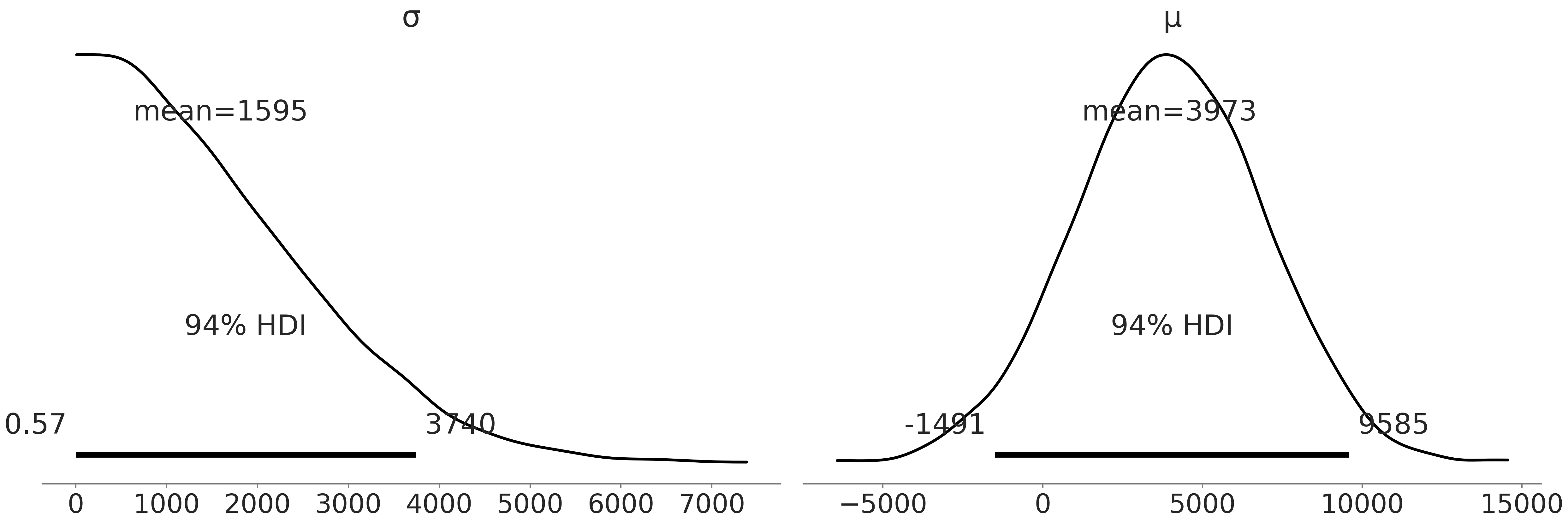
Fig. 3.1 Prior samples generated in Code Block penguin_mass. The distribution estimates of both the mean and standard deviation for the mass distribution cover a wide range of possibilities.

After sampling from our model, we can create Fig. 3.2 which includes 4 subplots, the two on the right are the rank plots and the left the KDE of each parameter, one line for each chain. We also can reference the numerical diagnostics in Table 3.2 to confirm our belief that the chains converged. Using the intuition we built in Chapter 2 we can judge that these fits are acceptable and we will continue with our analysis.

Table 3.2 Bayesian estimates of the mean (μ) and standard deviation (σ) of Adelie penguin mass. Sampling diagnostics also included

	mean	sd	hdi_3%	hdi_97%	mcse_mean	mcse_sd	ess_bulk	ess_tail	r_hat
\(\mu\)	3707	38	3632	3772	0.6	0.4	3677.0	2754.0	1.0
\(\sigma\)	463	27	401	511	0.5	0.3	3553.0	2226.0	1.0

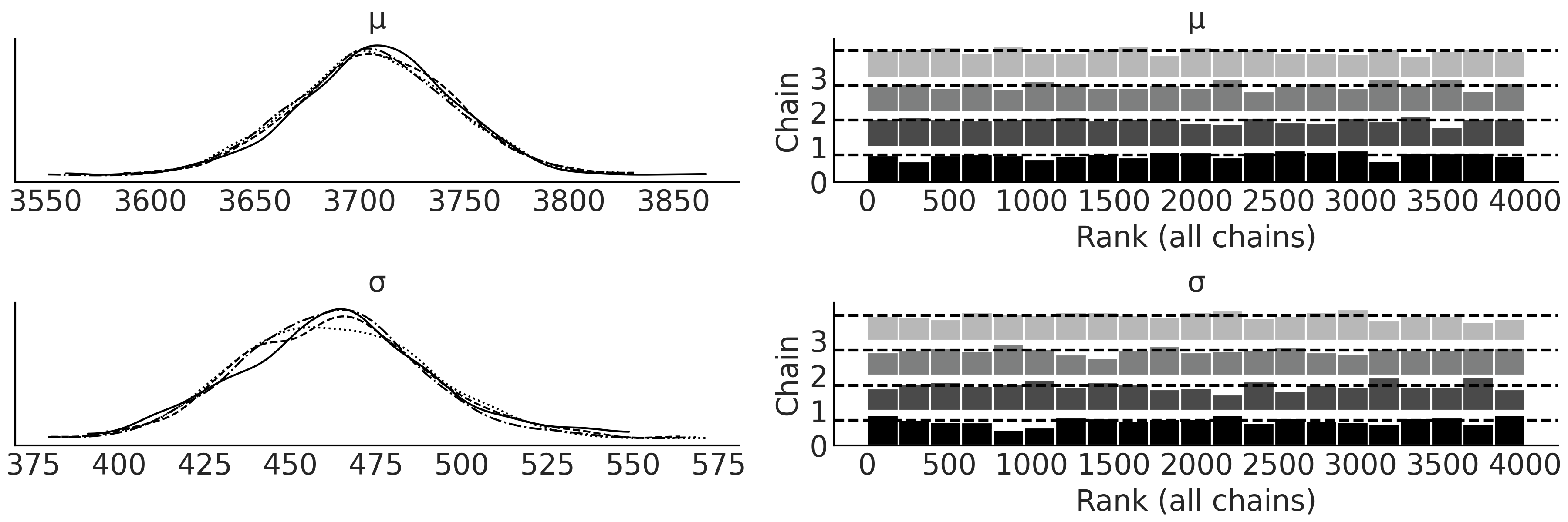
Fig. 3.2 KDE and rank plot of the posterior of the Bayesian model in Code Block penguin_mass of Adelie penguin mass. This plot serves as a visual diagnostic of the sampling to help judge if there were any issues during sampling across the multiple sampling chains.

Comfortable with the fit we plot a posterior plot in Fig. 3.3 that combines all the chains. Compare the point estimates from Table 3.1 of the mean and standard deviation with our Bayesian estimates as shown in Fig. 3.3.

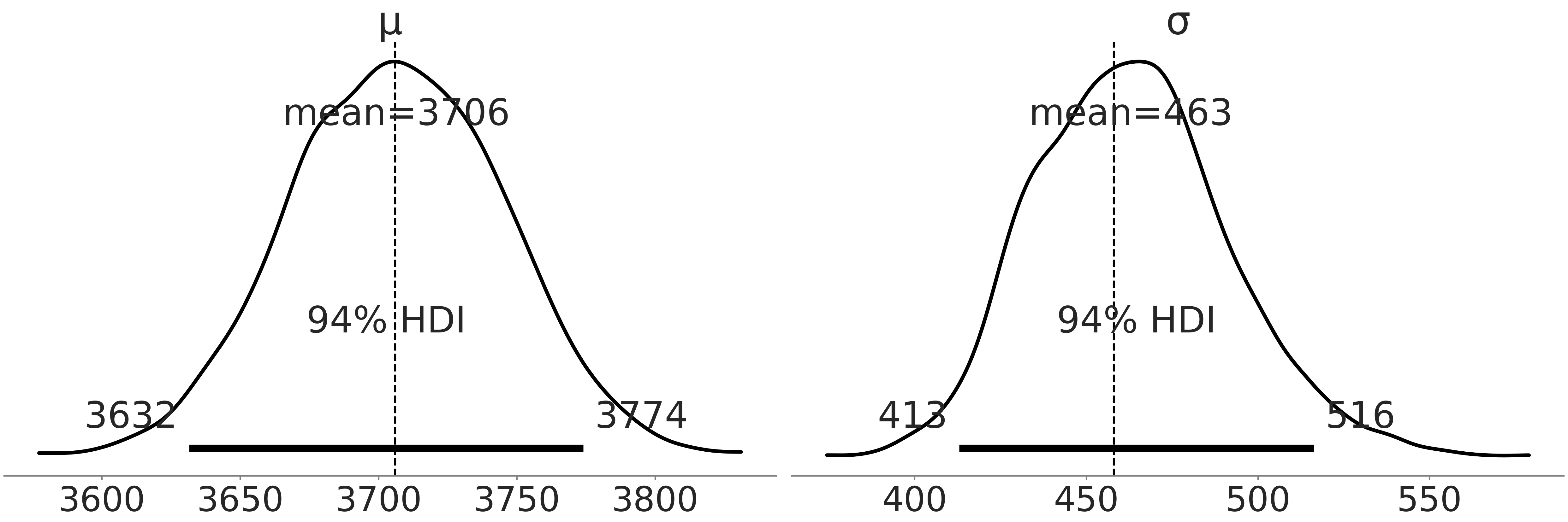
Fig. 3.3 Posterior plot of the posterior of the Bayesian model in Code Block penguin_mass of Adelie penguins mass. The vertical lines are the empirical mean and standard deviation.

With the Bayesian estimate however, we also get the distribution of plausible parameters. Using the tabular summary in Table Table 3.2 from the same posterior distribution in Fig. 3.2 values of the mean from 3632 to 3772 grams are quite plausible. Note that the standard deviation of the marginal posterior distribution varies quite a bit as well. And remember the posterior distribution is not the distribution of an individual penguin mass but rather possible parameters of a Gaussian distribution that we assume describes penguin mass. If we wanted the estimated distribution of individual penguin mass we would need to generate a posterior predictive distribution. In this case it will be the same Gaussian distribution conditioned on the posterior of \(\mu\) and \(\sigma\).

Now that we have characterized the Adelie penguin’s mass, we can do the same for the other species. We could do so by writing two more models but instead let us just run one model with 3 separated groups, one per species.

Listing 3.4 nocovariate_mass

# pd.categorical makes it easy to index species below
all_species = pd.Categorical(penguins["species"])

with pm.Model() as model_penguin_mass_all_species:
    # Note the addition of the shape parameter
    σ = pm.HalfStudentT("σ", 100, 2000, shape=3)
    μ = pm.Normal("μ", 4000, 3000, shape=3)
    mass = pm.Normal("mass",
                     mu=μ[all_species.codes],
                     sigma=σ[all_species.codes],
                     observed=penguins["body_mass_g"])

    trace = pm.sample()
    inf_data_model_penguin_mass_all_species = az.from_pymc3(
        trace=trace,
        coords={"μ_dim_0": all_species.categories,
                "σ_dim_0": all_species.categories})

We use the optional shape argument in each parameter and add an index in our likelihood indicating to PyMC3 that we want to condition the posterior estimate for each species individually. In programming language design small tricks that make expressing ideas more seamless are called syntactic sugar, and probabilistic programming developers include these as well. Probabilistic Programming Languages strive to allow expressing models with ease and with less errors.

After we run the model we once again inspect the KDE and rank plots, see Fig. 3.4. Compared to Fig. 3.2 you will see 4 additional plots, 2 each for the additional parameters added. Take a moment to compare the estimate of the mean with the summary mean shown for each species in Table 3.1. To better visualize the differences between the distributions for each species, we plot the posterior again in a forest plot using Code Block mass_forest_plot. Fig. 3.5 makes it easier to compare our estimates across species and note that the Gentoo penguins seem to have more mass than Adelie or Chinstrap penguins.

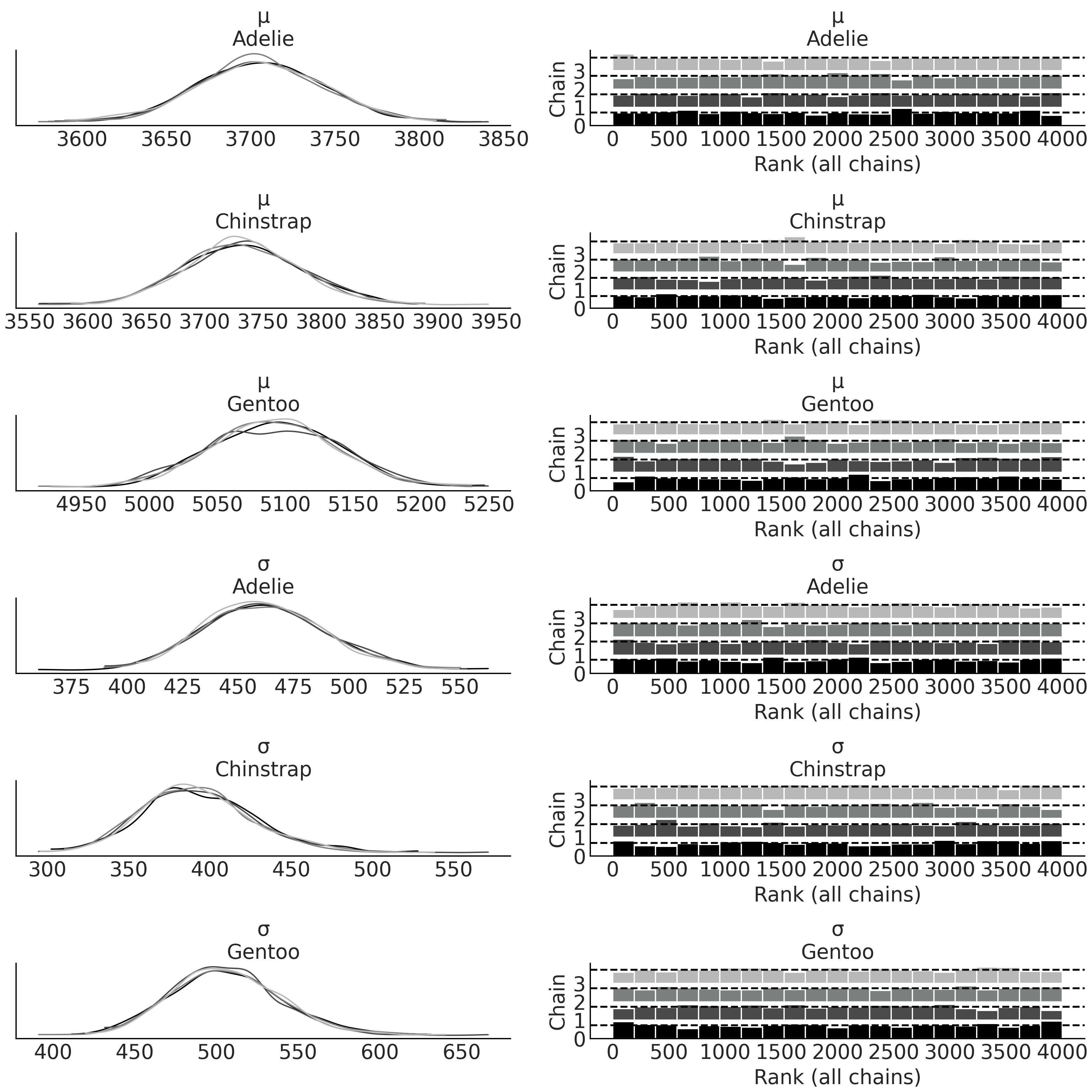
Fig. 3.4 KDE and rank plot for posterior estimates of parameters of masses for each species of penguins from the penguins_masses model. Note how each species has its own pair of estimates for each parameter.

Listing 3.5 mass_forest_plot

az.plot_forest(inf_data_model_penguin_mass_all_species, var_names=["μ"])

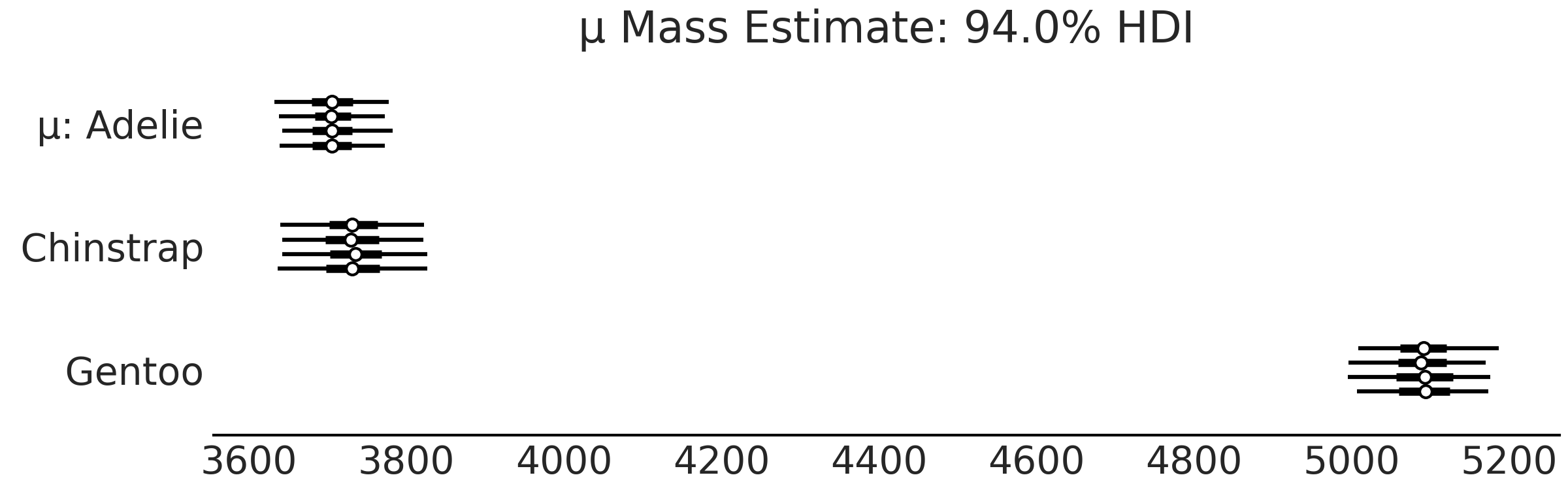
Fig. 3.5 Forest plot of the mean of mass of each species group in model_penguin_mass_all_species. Each line represents one chain in the sampler, the dot is the mean, the thick line is the interquartile range and the thin line is the 94% Highest Density Interval.

Fig. 3.5 makes it easier to compare our estimates and easily note that the Gentoo penguins have more mass than Adelie or Chinstrap penguins. Let us also look at the standard deviation in Fig. 3.6. The 94% highest density interval of the posterior is reporting uncertainty in the order of 100 grams.

az.plot_forest(inf_data_model_penguin_mass_all_species, var_names=["σ"])

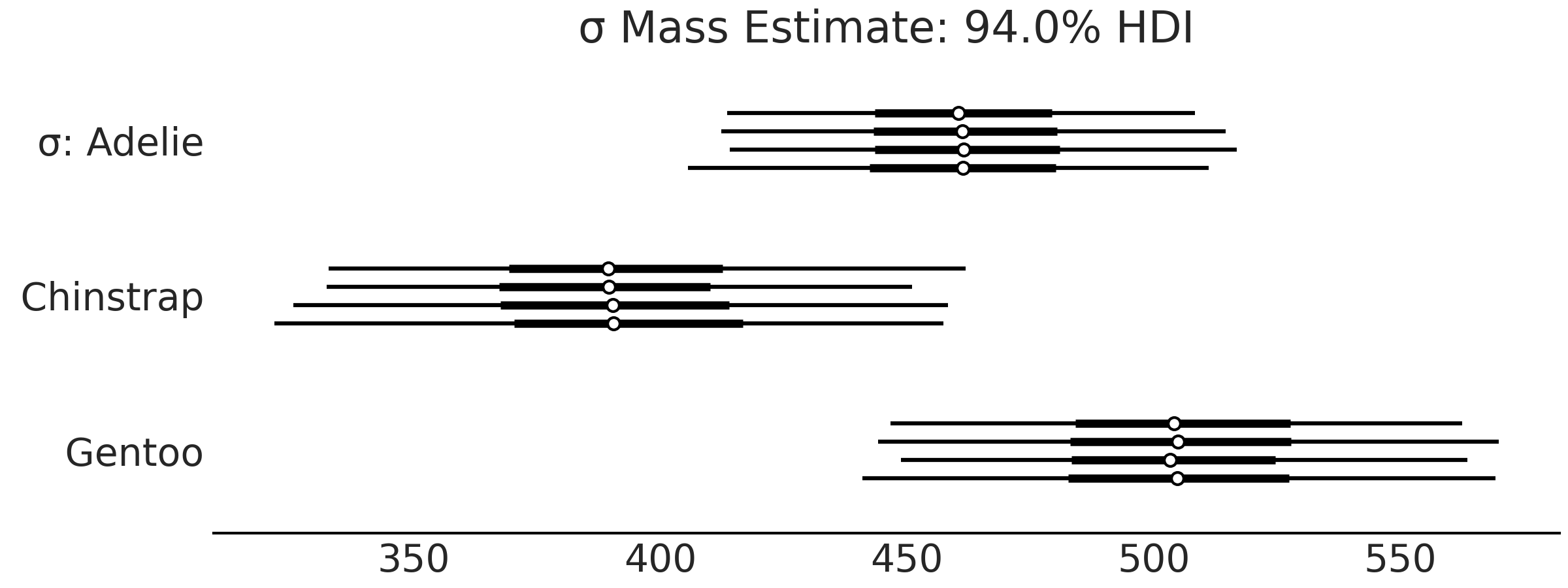
Fig. 3.6 Forest plot of the standard deviations of the mass for each species group in model_penguin_mass_all_species. This plot depicts our estimation of the dispersion of penguin mass, so for example, given a mean estimate of the Gentoo penguin distribution, the associated standard deviation is plausibly anywhere between 450 grams to 550 grams.

3.1.1. Comparing Two PPLs

Before expanding on the statistical and modeling ideas further, we will take a moment to talk about the probabilistic programming languages and introduce another PPL we will be using in this book, TensorFlow Probability (TFP). We will do so by translating the PyMC3 intercept only model in Code Block nocovariate_mass into TFP.

It may seem unnecessary to learn different PPLs. However, there are specific reasons we chose to use two PPLs instead of one in this book. Seeing the same workflow in different PPLs will give you a more thorough understanding of computational Bayesian modeling, help you separate computational details from statistical ideas, and make you a stronger modeler overall. Moreover, different PPLs have different strength and focus. PyMC3 is a higher level PPL that makes it easier to express models with less code, whereas TFP provides a lower level PPL for composable modeling and inference. Another is that not all PPLs are able to express all models as easily as each other. For instance Time Series models (Chapter 6) are more easily defined in TFP whereas Bayesian Additive Regression Trees are more easily expressed in PyMC3 (Chapter 7). Through this exposure to multiple languages you will come out with a stronger understanding of both the fundamental elements of Bayesian modeling and how they are implemented computationally.

Probabilistic Programming Languages (emphasis on language) are composed of primitives. The primitives in a programming language are the simplest elements available to construct more complex programs. You can think of primitives are like words in natural languages which can form more complex structures, like sentences. And as different languages use different words, different PPLs use different primitives. These primitives are mainly used to express models, perform inference, or express other parts of the workflow. In PyMC3, model building related primitives are contained under the namespace pm. For example, in Code Block penguin_mass we see pm.HalfStudentT(.), and pm.Normal(.), which represent a random variable. The with pm.Model() as . statement evokes a Python context manager, which PyMC3 uses to build the model model_adelie_penguin_mass by collecting the random variables within the context manager. We then use pm.sample_prior_predictive(.) and pm.sample(.) to obtain samples from the prior predictive distribution and from the posterior distribution, respectively.

Similarly, TFP provides primitives for user to specify distributions and model in tfp.distributions, running MCMC (tfp.mcmc), and more. For example, to construct a Bayesian model, TensorFlow provides multiple primitives under the name tfd.JointDistribution [29] API. In this chapter and the remaining of the book we mostly use tfd.JointDistributionCoroutine, but there are other variants of tfd.JointDistribution which may better suit your use case [1]. Since basic data import and summary statistics stays the same as Code Block penguin_load and penguin_mass_empirical we can focus on the model building and inference. model_penguin_mass_all_species expressed in TFP which is shown in Code Block penguin_mass_tfp below

Listing 3.6 penguin_mass_tfp

import tensorflow as tf
import tensorflow_probability as tfp

tfd = tfp.distributions
root = tfd.JointDistributionCoroutine.Root

species_idx = tf.constant(all_species.codes, tf.int32)
body_mass_g = tf.constant(penguins["body_mass_g"], tf.float32)

@tfd.JointDistributionCoroutine
def jd_penguin_mass_all_species():
    σ = yield root(tfd.Sample(
            tfd.HalfStudentT(df=100, loc=0, scale=2000),
            sample_shape=3,
            name="sigma"))
    μ = yield root(tfd.Sample(
            tfd.Normal(loc=4000, scale=3000),
            sample_shape=3,
            name="mu"))
    mass = yield tfd.Independent(
        tfd.Normal(loc=tf.gather(μ, species_idx, axis=-1),
                   scale=tf.gather(σ, species_idx, axis=-1)),
        reinterpreted_batch_ndims=1,
        name="mass")

Since this is our first encounter with a Bayesian model written in TFP, let us spend a few paragraphs to detail the API. The primitives are distribution classes in tfp.distributions, which we assign a shorter alias tfd = tfp.distributions. tfd contains commonly used distributions like tfd.Normal(.). We also used tfd.Sample, which returns multiple independent copies of the base distribution (conceptually we achieve the similar goal as using the syntactic sugar shape=(.) in PyMC3). tfd.Independent is used to indicate that the distribution contains multiple copies that we would like to sum over some axis when computing the log-likelihood, which specified by the reinterpreted_batch_ndims function argument. Usually we wrap the distributions associated with the observation with tfd.Independent [2]. You can read a bit more about shape handling in TFP and PPL in Section Shape Handling in PPLs.

An interesting signature of a tfd.JointDistributionCoroutine model is, as the name suggests, the usage of Coroutine in Python. Without getting into too much detail about Generators and Coroutines, here a yield statement of a distribution gives you some random variable inside of your model function. You can view y = yield Normal(.) as the way to express \(y \sim \text{Normal(.)}\). Also, we need to identify the random variables without dependencies as root nodes by wrapping them with tfd.JointDistributionCoroutine.Root. The model is written as a Python function with no input argument and no return value. Lastly, it is convenient to put @tfd.JointDistributionCoroutine on top of the Python function as a decorator to get the model (i.e., a tfd.JointDistribution) directly.

The resulting jd_penguin_mass_all_species is the intercept only regression model in Code Block nocovariate_mass restated in TFP. It has similar methods like other tfd.Distribution, which we can utilize in our Bayesian workflow. For example, to draw prior and prior predictive samples, we can call the .sample(.) method, which returns a custom nested Python structure similar to a namedtuple. In Code Block penguin_mass_tfp_prior_predictive we draw 1000 prior and prior predictive samples.

Listing 3.7 penguin_mass_tfp_prior_predictive

prior_predictive_samples = jd_penguin_mass_all_species.sample(1000)

The .sample(.) method of a tfd.JointDistribution can also draw conditional samples, which is the mechanism we will make use of to draw posterior predictive samples. You can run Code Block penguin_mass_tfp_prior_predictive2 and inspect the output to see how random samples change if you condition some random variables in the model to some specific values. Overall, we invoke the forward generative process when calling .sample(.).

Listing 3.8 penguin_mass_tfp_prior_predictive2

jd_penguin_mass_all_species.sample(sigma=tf.constant([.1, .2, .3]))
jd_penguin_mass_all_species.sample(mu=tf.constant([.1, .2, .3]))

Once we condition the generative model jd_penguin_mass_all_species to the observed penguin body mass, we can get the posterior distribution. From the computational perspective, we want to generate a function that returns the posterior log-probability (up to some constant) evaluated at the input. This could be done by creating a Python function closure or using the .experimental_pin method, as shown in Code Block tfp_posterior_generation:

Listing 3.9 tfp_posterior_generation

target_density_function = lambda *x: jd_penguin_mass_all_species.log_prob(
    *x, mass=body_mass_g)

jd_penguin_mass_observed = jd_penguin_mass_all_species.experimental_pin(
    mass=body_mass_g)
target_density_function = jd_penguin_mass_observed.unnormalized_log_prob

Inference is done using target_density_function, for example, we can find the maximum of the function, which gives the maximum a posteriori probability (MAP) estimate. We can also use methods in tfp.mcmc [30] to sample from the posterior. Or more conveniently, using a standard sampling routine similar to what is currently used in PyMC3 [3] as shown in Code Block tfp_posterior_inference:

Listing 3.10 tfp_posterior_inference

run_mcmc = tf.function(
    tfp.experimental.mcmc.windowed_adaptive_nuts,
    autograph=False, jit_compile=True)
mcmc_samples, sampler_stats = run_mcmc(
    1000, jd_penguin_mass_all_species, n_chains=4, num_adaptation_steps=1000,
    mass=body_mass_g)

inf_data_model_penguin_mass_all_species2 = az.from_dict(
    posterior={
        # TFP mcmc returns (num_samples, num_chains, ...), we swap
        # the first and second axis below for each RV so the shape
        # is what ArviZ expected.
        k:np.swapaxes(v, 1, 0)
        for k, v in mcmc_samples._asdict().items()},
    sample_stats={
        k:np.swapaxes(sampler_stats[k], 1, 0)
        for k in ["target_log_prob", "diverging", "accept_ratio", "n_steps"]}
)

In Code Block tfp_posterior_inference we ran 4 MCMC chains, each with 1000 posterior samples after 1000 adaptation steps. Internally it invokes the experimental_pin method by conditioning the model (pass into the function as an argument) with the observed (additional keyword argument mass=body_mass_g at the end). Lines 8-18 parse the sampling result into an ArviZ InferenceData, which we can now run diagnostics and exploratory analysis of Bayesian models in ArviZ. We can additionally add prior and posterior predictive samples and data log-likelihood to inf_data_model_penguin_mass_all_species2 in a transparent way in Code Block tfp_idata_additional below. Note that we make use of the sample_distributions method of a tfd.JointDistribution that draws samples and generates a distribution conditioned on the posterior samples.

Listing 3.11 tfp_idata_additional

prior_predictive_samples = jd_penguin_mass_all_species.sample([1, 1000])
dist, samples = jd_penguin_mass_all_species.sample_distributions(
    value=mcmc_samples)
ppc_samples = samples[-1]
ppc_distribution = dist[-1].distribution
data_log_likelihood = ppc_distribution.log_prob(body_mass_g)

# Be careful not to run this code twice during REPL workflow.
inf_data_model_penguin_mass_all_species2.add_groups(
    prior=prior_predictive_samples[:-1]._asdict(),
    prior_predictive={"mass": prior_predictive_samples[-1]},
    posterior_predictive={"mass": np.swapaxes(ppc_samples, 1, 0)},
    log_likelihood={"mass": np.swapaxes(data_log_likelihood, 1, 0)},
    observed_data={"mass": body_mass_g}
)

This concludes our whirlwind tour of TensorFlow Probability. Like any language you likely will not gain fluency in your initial exposure. But by comparing the two models you should now have a better sense of what concepts are Bayesian centric and what concepts are PPL centric. For the remainder of this chapter and the next we will switch between PyMC3 and TFP to continue helping you identify this difference and see more worked examples. We include exercises to translate Code Block examples from one to the other to aid your practice journey in becoming a PPL polyglot.

3.2. Linear Regression

In the previous section we modeled the distribution of penguin mass by setting prior distributions over the mean and standard deviation of a Gaussian distribution. Importantly we assumed that the mass did not vary with other features in the data. However, we would expect that other observed data points could provide information about expected penguins mass. Intuitively if we see two penguins, one with long flippers and one with short flippers, we would expect the larger penguin, the one with long flippers, to have more mass even if we did not have a scale on hand to measure their mass precisely. One of the simplest ways to estimate this relationship of observed flipper length on estimated mass is to fit a linear regression model, where the mean is conditionally modeled as a linear combination of other variables

(3.2)\[\begin{split}\begin{split} \mu =& \beta_0 + \beta_1 X_1 + \dots + \beta_m X_m \\ Y \sim& \mathcal{N}(\mu, \sigma) \end{split}\end{split}\]

where the coefficients, also referred as parameters, are represented with \(\beta_i\). For example, \(\beta_0\) is the intercept of the linear model. \(X_i\) is referred to predictors or independent variables, and \(Y\) is usually referred to as target, output, response, or dependent variable. It is important to notice that both \(\boldsymbol{X}\) and \(Y\) are observed data and that they are paired \(\{y_j, x_j\}\). That is, if we change the order of \(Y\) without changing \(X\) we will destroy some of the information in our data.

We call this a linear regression because the parameters (not the covariates) enter the model in a linear fashion. Also for models with a single covariate, we can think of this model as fitting a line to the \((X, y)\) data, and for higher dimensions a plane or more generally a hyperplane.

Alternatively we can express Equation (3.2) using matrix notation:

(3.3)\[\mu = \mathbf{X}\boldsymbol{\beta}\]

where we are taking the matrix-vector product between the coefficient column vector \(\beta\) and the matrix of covariates \(\mathbf{X}\).

An alternative expression you might have seen in other (non-Bayesian) occasions is to rewrite Equation (3.2) as noisy observation of some linear prediction:

(3.4)\[Y = \mathbf{X}\boldsymbol{\beta} + \epsilon,\; \epsilon \sim \mathcal{N}(0, \sigma)\]

The formulation in Equation (3.4) separates the deterministic part (linear prediction) and the stochastic part (noise) of linear regression. However, we prefer Equation (3.2) as it shows the generative process more clearly.

Design Matrix

The matrix \(\mathbf{X}\) in Equation (3.3) is known as design matrix and is a matrix of values of explanatory variables of a given set of objects, plus an additional column of ones to represent the intercept. Each row represents an unique observation (e.g., a penguin), with the successive columns corresponding to the variables (like flipper length) and their specific values for that object.

A design matrix is not limited to continuous covariates. For discrete covariates that represent categorical predictors (i.e., there are only a few categories), a common way to turn those into a design matrix is called dummy coding or one-hot coding. For example, in our intercept per penguin model (Code Block nocovariate_mass), instead of mu = μ[species.codes] we can use pandas.get_dummies to parse the categorical information into a design matrix, and then write mu = pd.get_dummies(penguins["species"]) @ μ, where @ is a Python operator for performing matrix multiplication. There are also few other functions to perform one hot encoding in Python, for example, sklearn.preprocessing.OneHotEncoder, as this is a very common data manipulation technique.

Alternatively, categorical predictors could be encoded such that the resulting column and associated coefficient representing linear contrast. For example, different design matrix encoding of two categorical predictors are associated with Type I, II and III sums of squares in null-hypothesis testing setting for ANOVA.

If we plot Equation (3.2) in “three dimensions” we get Fig. 3.7, which shows how the estimated parameters of the likelihood distribution can change based on other observed data \(x\). While in this one illustration, and in this chapter, we are using a linear relationship to model the relationship between \(x\) and \(Y\), and a Gaussian distribution as a likelihood, in other model architectures, we may opt for different choices as we will see in Chapter 4.

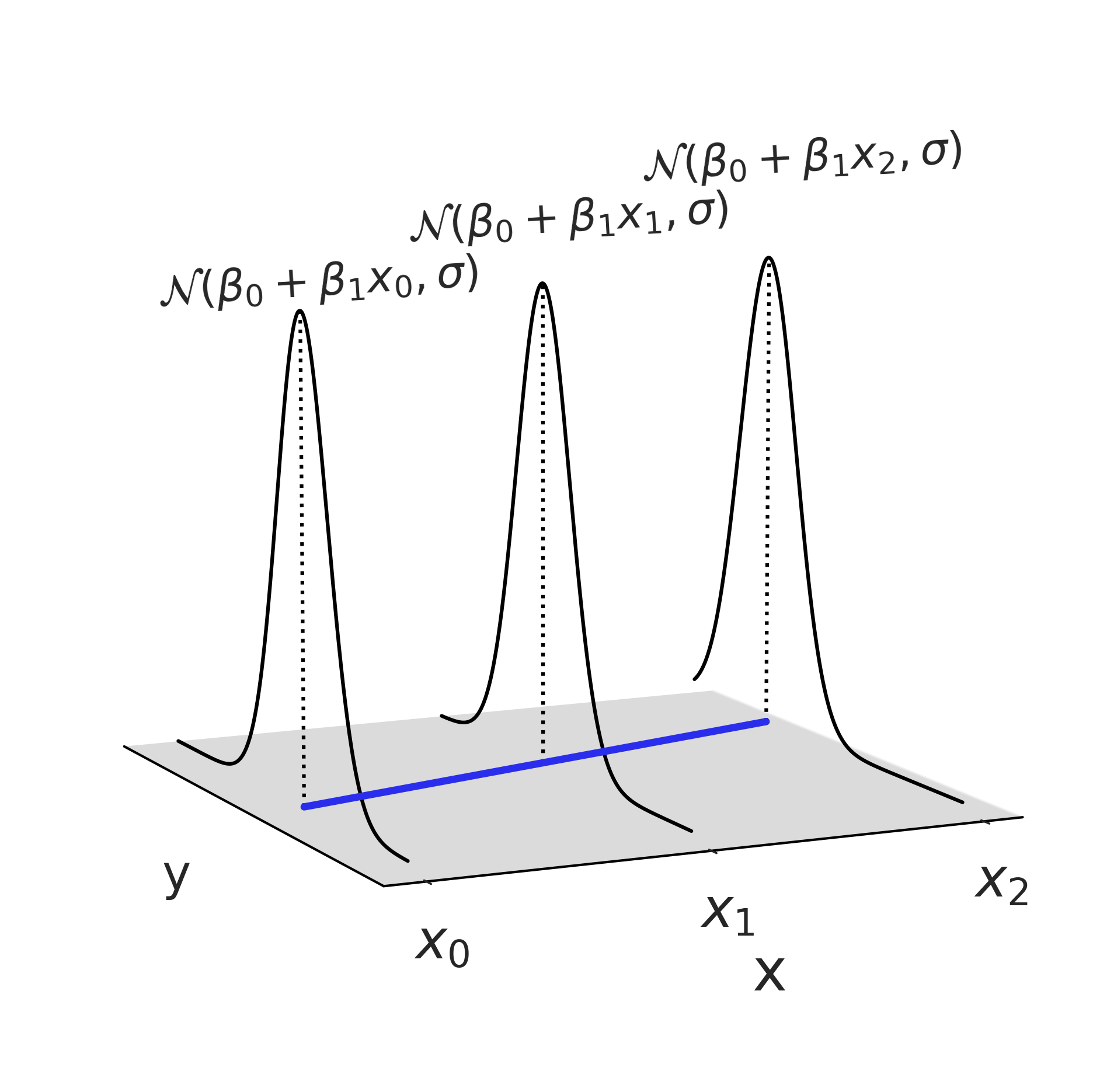
Fig. 3.7 A linear regression with the Gaussian likelihood function evaluated at 3 points. Note this plot only shows one possible Gaussian distribution at each value of \(x\), where after fitting a Bayesian model we will end up with a distribution of Gaussian, whose parameters may follow a distribution other than Gaussian.

3.2.1. Linear Penguins

If we recall our penguins we were interested using additional data to better estimate the mean mass of a group of penguins. Using linear regression we write the model in Code Block non_centered_regression, which includes two new parameters \(\beta_0\) and \(\beta_1\) typically called the intercept and slope. For this example we set wide priors of \(\mathcal{N}(0, 4000)\) to focus on the model, which also is the same as saying we assume no domain expertise. We subsequently run our sampler, which has now estimated three parameters \(\sigma\), \(\beta_1\) and \(\beta_0\).

Listing 3.12 non_centered_regression

adelie_flipper_length_obs = penguins.loc[adelie_mask, "flipper_length_mm"]

with pm.Model() as model_adelie_flipper_regression:
    # pm.Data allows us to change the underlying value in a later code block
    adelie_flipper_length = pm.Data("adelie_flipper_length",
                                    adelie_flipper_length_obs)
    σ = pm.HalfStudentT("σ", 100, 2000)
    β_0 = pm.Normal("β_0", 0, 4000)
    β_1 = pm.Normal("β_1", 0, 4000)
    μ = pm.Deterministic("μ", β_0 + β_1 * adelie_flipper_length)

    mass = pm.Normal("mass", mu=μ, sigma=σ, observed = adelie_mass_obs)

    inf_data_adelie_flipper_regression = pm.sample(return_inferencedata=True)

To save space in the book we are not going to show the diagnostics each time but you should neither trust us or your sampler blindly. Instead you should run the diagnostics to verify you have a reliable posterior approximation.

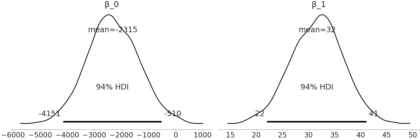
Fig. 3.8 Estimates of the parameter value distributions of our linear regression coefficient from model_adelie_flipper_regression.

After our sampler finishes running we can plot Fig. 3.8 which shows a full posterior plot we can use to inspect \(\beta_0\) and \(\beta_1\). The coefficient \(\beta_1\) expresses that for every millimeter change of Adelie flipper length we can nominally expect a change of 32 grams of mass, although anywhere between 22 grams to 41 grams could reasonably occur as well. Additionally, from Fig. 3.8 we can note how the 94% highest density interval does not cross 0 grams. This supports our assumption that there is a relationship between mass and flipper length. This observation is quite useful for interpreting how flipper length and mass correlate. However, we should be careful about not over-interpreting the coefficients or thinking a linear model necessarily implies a causal link. For example, if we perform a flipper extension surgery to a penguin this will not necessarily translate into a gain in mass, it could actually be the opposite due to stress or impediments of this penguin to get food. The opposite relation is not necessarily true either, providing more food to a penguin could help her to have a larger flipper, but it could also make it just a fatter penguin. Now focusing on \(\beta_0\) however, what does it represent? From our posterior estimate we can state that if we saw an Adelie penguin with a 0 mm flipper length we would expect the mass of this impossible penguin to be somewhere between -4151 and -510 grams. According to our model this statement is true, but negative mass does not make sense. This is not necessarily an issue, there is no rule that every parameter in a model needs to be interpretable, nor that the model provide reasonable prediction at every parameter value. At this point in our journey the purpose of this particular model was to estimate the relationship between flipper length and penguin mass and with our posterior estimates, we have succeeded with that goal.

Models: A balance between math and reality

In our penguin example it would not make sense if penguin mass was below 0 (or even close to it), even though the model allowed it. Because we fit the model using values for the masses that are far from 0, we should not be surprised that the model fails if we want to extrapolate conclusions for values close to 0 or below it. A model does not necessarily have to provide sensible predictions for all possible values, it just needs to provide sensible predictions for the purposes that we are building it for.

We started on this section surmising that incorporating a covariate would lead to better predictions of penguin mass. We can verify this is the case by comparing the posterior estimates of \(\sigma\) from our fixed mean model and with our linearly varying mean model in Fig. 3.9, our estimate of the likelihood’s standard deviation has dropped from a mean of around \(\approx 460\) grams to \(\approx 380\) grams.

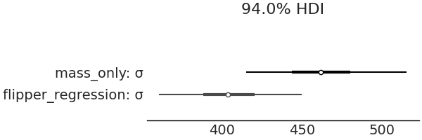
Fig. 3.9 By using the covariate of flipper length when estimating penguin mass the magnitude of the estimated error is reduced from a mean of slightly over 460 grams to around 380 grams. This intuitively makes sense as if we are given information about a quantity we are estimating, we can leverage that information to make better estimates.

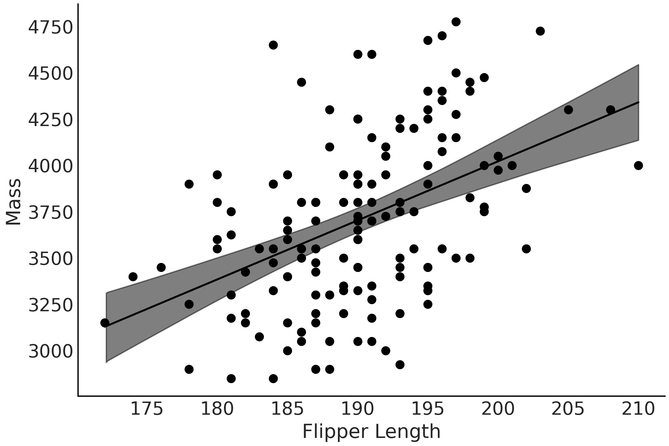
Fig. 3.10 Observed Adelie data of flipper length vs mass as scatter plot, and mean estimate of the likelihood as black line, and 94% HDI of the mean as gray interval. Note how our mean estimate varies as flipper varies.

3.2.2. Predictions

In the Linear Penguins we estimated a linear relationship between flipper length and mass. Another use of regression is to leverage that relationship in order to make predictions. In our case given the flipper length of a penguin, can we predict its mass? In fact we can. We will use our results from model_adelie_flipper_regression to do so. Because in Bayesian statistics we are dealing with distributions we do not end up with a single predicted value but instead a distribution of possible values. That is the posterior predictive distribution as defined in Equation (1.8). In practice, more often than not, we will not compute our predictions analytically but we will use a PPL to estimate them using our posterior samples. For example, if we had a penguin of average flipper length and wanted to predict the likely mass using PyMC3 we would write Code Block penguins_ppd:

Listing 3.13 penguins_ppd

with model_adelie_flipper_regression:
    # Change the underlying value to the mean observed flipper length
    # for our posterior predictive samples
    pm.set_data({"adelie_flipper_length": [adelie_flipper_length_obs.mean()]})
    posterior_predictions = pm.sample_posterior_predictive(
        inf_data_adelie_flipper_regression.posterior, var_names=["mass", "μ"])

In the first line of Code Block penguins_ppd we fix the value of our flipper length to the average observed flipper length. Then using the regression model model_adelie_flipper_regression, we can generate posterior predictive samples of the mass at that fixed value. In Fig. 3.11 we plot the posterior predictive distribution of the mass for penguins of average flipper length, along the posterior of the mean.

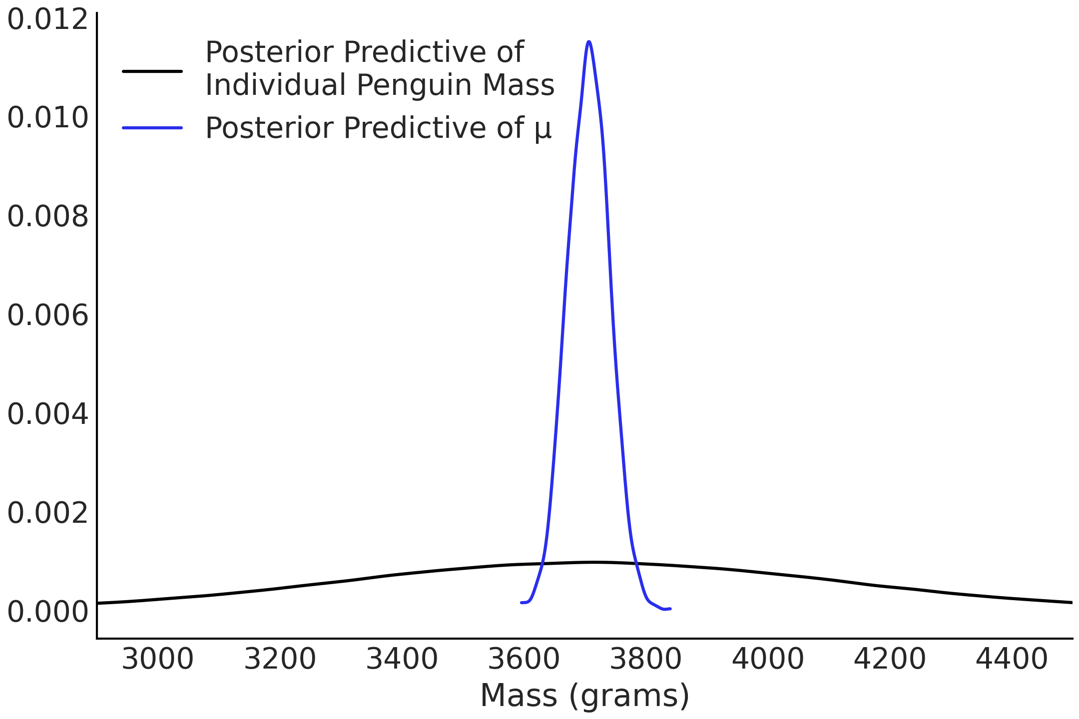
Fig. 3.11 The posterior distribution of the mean, \(\mu\), evaluated at the mean flipper length in blue and the posterior predictive distribution evaluated at the mean flipper length in black. The black curve is wider as it describes the distribution of the predicted data (for a given flipper length), while the blue curve represents the distribution of just the mean of the predicted data.

In short not only can we use our model in Code Block non_centered_regression to estimate the relationship between flipper length and mass, we also can obtain an estimate of the penguin mass at any arbitrary flipper length. In other words we can use the estimated \(\beta_1\) and \(\beta_0\) coefficients to make predictions of the mass of unseen penguins of any flipper length using posterior predictive distributions.

As such, the posterior predictive distribution is an especially powerful tool in a Bayesian context as it let us predict not just the most likely value, but a distribution of plausible values incorporating the uncertainty about our estimates, as seen from Equation (1.8).

3.2.3. Centering

Our model in Code Block non_centered_regression worked well for estimating the correlation between flipper length and penguin mass, and in predicting the mass of penguins at a given flipper length. Unfortunately with the data and the model provided our estimate of \(\beta_0\) was not particularly useful. However, we can use a transformation to make \(\beta_0\) more interpretable. In this case we will opt for a centering transformation, which takes a set of values and centers its mean value at zero as shown in Code Block flipper_centering.

Listing 3.14 flipper_centering

adelie_flipper_length_c = (adelie_flipper_length_obs -
                           adelie_flipper_length_obs.mean())

With our now centered covariate let us fit our model again, this time using TFP.

Listing 3.15 tfp_penguins_centered_predictor

def gen_adelie_flipper_model(adelie_flipper_length):
    adelie_flipper_length = tf.constant(adelie_flipper_length, tf.float32)

    @tfd.JointDistributionCoroutine
    def jd_adelie_flipper_regression():
        σ = yield root(
            tfd.HalfStudentT(df=100, loc=0, scale=2000, name="sigma"))
        β_1 = yield root(tfd.Normal(loc=0, scale=4000, name="beta_1"))
        β_0 = yield root(tfd.Normal(loc=0, scale=4000, name="beta_0"))
        μ = β_0[..., None] + β_1[..., None] * adelie_flipper_length
        mass = yield tfd.Independent(
            tfd.Normal(loc=μ, scale=σ[..., None]),
            reinterpreted_batch_ndims=1,
            name="mass")

    return jd_adelie_flipper_regression

# If use non-centered predictor, this will give the same model as
# model_adelie_flipper_regression
jd_adelie_flipper_regression = gen_adelie_flipper_model(
    adelie_flipper_length_c)

mcmc_samples, sampler_stats = run_mcmc(
    1000, jd_adelie_flipper_regression, n_chains=4, num_adaptation_steps=1000,
    mass=tf.constant(adelie_mass_obs, tf.float32))

inf_data_adelie_flipper_length_c = az.from_dict(
    posterior={
        k:np.swapaxes(v, 1, 0)
        for k, v in mcmc_samples._asdict().items()},
    sample_stats={
        k:np.swapaxes(sampler_stats[k], 1, 0)
        for k in ["target_log_prob", "diverging", "accept_ratio", "n_steps"]}
)

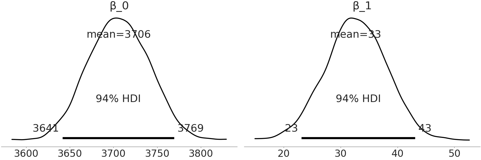
Fig. 3.12 Estimates of coefficients from Code Block tfp_penguins_centered_predictor. Notice that the distribution of \(beta\_1\) is the same as in Fig. 3.8, but the distribution of \(beta\_0\) has shifted. Because we centered the observations around the mean of flipper length \(beta\_0\) now represents the mass distribution of the average flipper penguin.

The mathematical model we defined in Code Block tfp_penguins_centered_predictor is identical to the PyMC3 model model_adelie_flipper_regression from Code Block non_centered_regression, with sole difference being the centering of the predictor. PPL wise however, the structure of TFP necessitates the addition of tensor_x[..., None] in various lines to extend a batch of scalars so that they are broadcastable with a batch of vectors. Specifically None appends a new axis, which could also be done using np.newaxis or tf.newaxis. We also wrap the model in a function so we can easily condition on different predictors. In this case we use the centered flipper length, but could also use the non-centered predictor which will yield similar results to our previous model.

When we plot our coefficients again, \(\beta_1\) is the same as our PyMC3 model but the distribution of \(\beta_0\) has changed. Since we have centered our input data on its mean, the distribution of \(\beta_0\) is the same as our prediction for the group mean with the non-centered dataset. By centering the data we now can directly interpret \(\beta_0\) as the distribution of mean masses for Adelie penguins with a mean flipper length. The idea of transforming the input variables can also be performed at arbitrary values of choice. For example, we could subtract out the minimum flipper length and fit our model. In this transformation this would change the interpretation \(\beta_0\) to the distribution of means for the smallest observed flipper length. For a greater discussion of transformations in linear regression we recommend Applied Regression Analysis and Generalized Linear Models [31].

3.3. Multiple Linear Regression

In many species there is a dimorphism, or difference, between different sexes. The study of sexual dimorphism in penguins actually was the motivating factor for collecting the Palmer Penguin dataset [32]. To study penguin dimorphism more closely let us add a second covariate, this time sex, encoding it as a categorical variable and seeing if we can estimate a penguins mass more precisely.

Listing 3.16 penguin_mass_multi

# Binary encoding of the categorical predictor
sex_obs = penguins.loc[adelie_mask ,"sex"].replace({"male":0, "female":1})

with pm.Model() as model_penguin_mass_categorical:
    σ = pm.HalfStudentT("σ", 100, 2000)
    β_0 = pm.Normal("β_0", 0, 3000)
    β_1 = pm.Normal("β_1", 0, 3000)
    β_2 = pm.Normal("β_2", 0, 3000)

    μ = pm.Deterministic(
        "μ", β_0 + β_1 * adelie_flipper_length_obs + β_2 * sex_obs)

    mass = pm.Normal("mass", mu=μ, sigma=σ, observed=adelie_mass_obs)

    inf_data_penguin_mass_categorical = pm.sample(
        target_accept=.9, return_inferencedata=True)

You will notice a new parameter, \(\beta_{2}\) contributing to the value of \(\mu\). As sex is a categorical predictor (in this example just female or male), we encode it as 1 and 0, respectively. For the model this means that the value of \(\mu\), for females, is a sum over 3 terms while for males is a sum of two terms (as the \(\beta_2\) term will zero out).

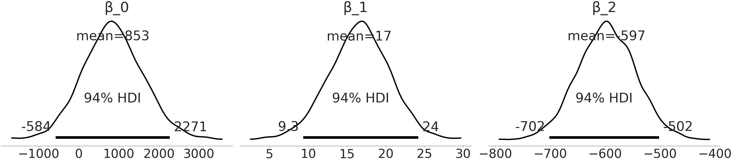
Fig. 3.13 Estimate of coefficient for sex covariate, \(\beta_{2}\) in model. As male is encoded as 0, and female is encoded as 1, this indicates the additional mass we would expect between a male and female Adelie penguin with the same flipper length.

Syntactic Linear Sugar

Linear models are so widely used that specialized syntax, methods, and libraries have been written just for regression. One such library is Bambi (BAyesian Model-Building Interface[33]). Bambi is a Python package for fitting generalized linear hierarchical models using a formula-based syntax, similar to what one might find in R packages, like lme4 [34], nlme [35], rstanarm [36] or brms [37]). Bambi uses PyMC3 underneath and provides a higher level API. To write the same model, if disregarding the priors[4] as the one in Code Block penguin_mass_multi in Bambi we would write:

Listing 3.17 bambi_categorical

import bambi as bmb
model = bmb.Model("body_mass_g ~ flipper_length_mm + sex",
                  penguins[adelie_mask])
trace = model.fit()

The priors are automatically assigned if not provided, as is the case in the code example above. Internally, Bambi stores virtually all objects generated by PyMC3, making it easy for users to retrieve, inspect, and modify those objects. Additionally Bambi returns an az.InferenceData object which can be directly used with ArviZ.

Since we have encoded male as 0 this posterior from model_penguin_mass_categorical estimates the difference in mass compared to a female Adelie penguin with the same flipper length. This last part is quite important, by adding a second covariate we now have a multiple linear regression and we must use more caution when interpreting the coefficients. In this case, the coefficients provides the relationship of a covariate into the response variable, if all other covariates are held constant [5].

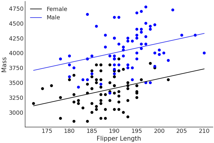
Fig. 3.14 Multiple regression for flipper length versus mass with male and female Adelie penguins coded as a categorical covariate. Note how the difference mass between male and female penguins is constant at every flipper length. This difference is equivalent to the magnitude of the \(\beta_2\) coefficient.

We again can compare the standard deviations across our three models in Fig. 3.15 to see if we have reduced uncertainty in our estimate and once again the additional information has helped to improve the estimate. In this case our estimate of \(\sigma\) has dropped a mean of 462 grams in our no covariate model defined in Code Block penguin_mass to a mean value 298 grams from the linear model defined in Code Block penguin_mass_multi that includes flipper length and sex as a covariates. This reduction in uncertainty suggests that sex does indeed provide information for estimating a penguin’s mass.

Listing 3.18 forest_multiple_models

az.plot_forest([inf_data_adelie_penguin_mass,
        inf_data_adelie_flipper_regression,
        inf_data_penguin_mass_categorical],
        var_names=["σ"], combined=True)

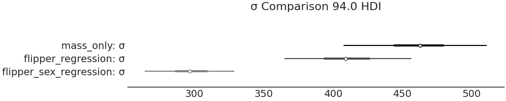
Fig. 3.15 By incorporating sex as a covariate in model_penguin_mass_categorical the estimated distribution of \(\sigma\) from this model is centered around 300 grams, which is a lower value than the estimated by our fixed mean model and our single covariate model. This figure is generated from Code Block forest_multiple_models.

More covariates is not always better

All model fitting algorithms will find a signal, even if it is random noise. This phenomenon is called overfitting and it describes a condition where the algorithm can quite handily map covariates to outcomes in seen cases, but fails to generalize to new observations. In linear regressions we can show this by generating 100 random covariates, and fitting them to a random simulated dataset [10]. Even though there is no relation, we would be led to believe our linear model is doing quite well.

3.3.1. Counterfactuals

In Code Block penguins_ppd we made a prediction using parameters fitted in a model with a single covariate and our target, and changing that covariate, flipper length, to get an estimate of mass at that fixed flipper length. In multiple regression, we can do something similar, where we take our regression, hold all covariates constant except one, and see how that change to that one covariate changes our expected outcome. This analysis is called a counterfactual analysis. Let us extend the multiple regression from the previous section (Code Block penguin_mass_multi), this time including bill length, and run a counterfactual analysis in TFP. The model building and inference is shown in Code Block tfp_flipper_bill_sex.

Listing 3.19 tfp_flipper_bill_sex

def gen_jd_flipper_bill_sex(flipper_length, sex, bill_length, dtype=tf.float32):
    flipper_length, sex, bill_length = tf.nest.map_structure(
        lambda x: tf.constant(x, dtype),
        (flipper_length, sex, bill_length)
    )

    @tfd.JointDistributionCoroutine
    def jd_flipper_bill_sex():
        σ = yield root(
            tfd.HalfStudentT(df=100, loc=0, scale=2000, name="sigma"))
        β_0 = yield root(tfd.Normal(loc=0, scale=3000, name="beta_0"))
        β_1 = yield root(tfd.Normal(loc=0, scale=3000, name="beta_1"))
        β_2 = yield root(tfd.Normal(loc=0, scale=3000, name="beta_2"))
        β_3 = yield root(tfd.Normal(loc=0, scale=3000, name="beta_3"))
        μ = (β_0[..., None]
             + β_1[..., None] * flipper_length
             + β_2[..., None] * sex
             + β_3[..., None] * bill_length
            )
        mass = yield tfd.Independent(
            tfd.Normal(loc=μ, scale=σ[..., None]),
            reinterpreted_batch_ndims=1,
            name="mass")

    return jd_flipper_bill_sex

bill_length_obs = penguins.loc[adelie_mask, "bill_length_mm"]
jd_flipper_bill_sex = gen_jd_flipper_bill_sex(
    adelie_flipper_length_obs, sex_obs, bill_length_obs)

mcmc_samples, sampler_stats = run_mcmc(
    1000, jd_flipper_bill_sex, n_chains=4, num_adaptation_steps=1000,
    mass=tf.constant(adelie_mass_obs, tf.float32))

In this model you will note the addition of another coefficient beta_3 to correspond to the addition of bill length as a covariate. After inference, we can simulate the mass of penguins with different fictional flipper lengths, while holding the sex constant at male, and the bill length at the observed mean of the dataset. This is done in Code Block tfp_flipper_bill_sex_counterfactuals with the result shown in Fig. 3.16. Again since we wrap the model generation in a Python function (a functional programming style approach), it is easy to condition on new predictors, which is useful for counterfactual analyses.

Listing 3.20 tfp_flipper_bill_sex_counterfactuals

mean_flipper_length = penguins.loc[adelie_mask, "flipper_length_mm"].mean()
# Counterfactual dimensions is set to 21 to allow us to get the mean exactly
counterfactual_flipper_lengths = np.linspace(
    mean_flipper_length-20, mean_flipper_length+20, 21)
sex_male_indicator = np.zeros_like(counterfactual_flipper_lengths)
mean_bill_length = np.ones_like(
    counterfactual_flipper_lengths) * bill_length_obs.mean()

jd_flipper_bill_sex_counterfactual = gen_jd_flipper_bill_sex(
    counterfactual_flipper_lengths, sex_male_indicator, mean_bill_length)
ppc_samples = jd_flipper_bill_sex_counterfactual.sample(value=mcmc_samples)
estimated_mass = ppc_samples[-1].numpy().reshape(-1, 21)

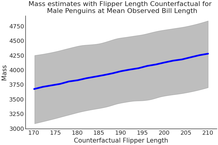
Fig. 3.16 Estimated counterfactual mass values for Adelie penguins from Code Block tfp_flipper_bill_sex_counterfactuals where flipper length is varied holding all other covariates constant.

Following McElreath[10] Fig. 3.16 is called a counterfactual plot. As the word counterfactual implies, we are evaluating a situation counter to the observed data, or facts. In other words, we are evaluating situations that have not happened. The simplest use of a counterfactual plot is to adjust a covariate and explore the result, exactly like we just did. This is great, as it enables us to explore what-if scenarios, that could be beyond our reach otherwise [6]. However, we must be cautious when interpreting this trickery. The first trap is that counterfactual values may be impossible, for example, no penguin may ever exist with a flipper length larger than 1500mm but the model will happily give us estimates for this fictional penguin. The second is more insidious, we assumed that we could vary each covariate independently, but in reality this may not be possible. For example, as a penguin’s flipper length increases, its bill length may as well. Counterfactuals are powerful in that they allow us to explore outcomes that have not happened, or that we at least did not observe happen. But they can easily generate estimates for situations that will never happen. It is the model that will not discern between the two, so you as a modeler must.

Correlation vs Causality

When interpreting linear regressions it is tempting to say “An increase in \(X\) causes and increase in \(Y\)”. This is not necessarily the case, in fact causal statements can not be made from a (linear) regression alone. Mathematically a linear model links two (or more variables) together but this link does not need to be causal. For example, increasing the amount of water we provide to a plant can certainly (and causally) increase the plant’s growth (at least within some range), but nothing prevents us from inverting this relationship in a model and use the growth of plants to estimate the amount of rain, even when plant growth do not cause rain [7]. The statistical sub-field of Causal Inference is concerned with the tools and procedures necessary to make causal statements either in the context of randomized experiments or observational studies (see Chapter 7 for a brief discussion)

3.4. Generalized Linear Models

All linear models discussed so far assumed the distribution of observations are conditionally Gaussian which works well in many scenarios. However, we may want to use other distributions. For example, to model things that are restricted to some interval, a number in the interval \([0, 1]\) like probabilities, or natural numbers \(\{1, 2, 3, \dots \}\) like counting events. To do this we will take our linear function, \(\mathbf{X} \mathit{\beta}\), and modify it using an inverse link function [8] \(\phi\) as shown in Equation (3.5).

(3.5)\[ \begin{align}\begin{aligned}\begin{split}\begin{split} \mu =& \phi(\mathbf{X} \beta) \\ Y \sim& \Psi (\mu, \theta)\end{split}\\\end{split}\end{aligned}\end{align} \]

where \(\Psi\) is some distribution parameterized by \(\mu\) and \(\theta\) indicating the data likelihood.

The specific purpose of the inverse link function is to map outputs from the range of real numbers \((-\infty, \infty)\) to a parameter range of the restricted interval. In other words the inverse link function is the specific “trick” we need to take our linear models and generalize them to many more model architectures. We are still dealing with a linear model here in the sense that the expectation of the distribution that generates the observation still follows a linear function of the parameter and the covariates but now we can generalize the use and application of these models to many more scenarios [9].

3.4.1. Logistic Regression

One of the most common generalized linear model is the logistic regression. It is particularly useful in modeling data where there are only two possible outcomes, we observed either one thing or another thing. The probability of a head or tails outcome in a coin flip is the usual textbook example. More “real world” examples includes the chance of a defect in manufacturing, a negative or positive cancer test, or the failure of a rocket launch [38]. In a logistic regression the inverse link function is called, unsurprisingly, the logistic function, which maps \((-\infty, \infty)\) to the \((0,1)\) interval. This is handy because now we can map linear functions to the range we would expect for a parameter that estimates probability values, that must be in the range 0 and 1 by definition.

(3.6)\[p = \frac{1}{1+e^{-\mathbf{X}\beta}}\]

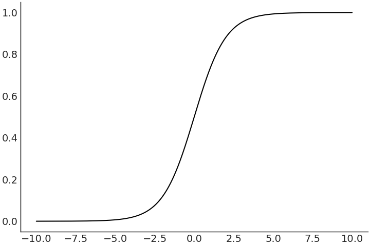
Fig. 3.17 A plot of a sample logistic function. Note the response has been “squished” into the interval (0,1).

With logistic regression we are able to use linear models to estimate probabilities of an event. Sometimes, instead we want to classify, or to predict, a specific class given some data. In order to do so we want to turn the continuous prediction in the interval \((-\infty, \infty)\) to one between 0 and 1. We can do this with a decision boundary to make a prediction in the set \({0,1}\). Let us assume we want our decision boundary set at a probability of 0.5. For a model with an intercept and one covariate we have:

(3.7)\[\begin{split}\begin{split} 0.5 &= logistic(\beta_{0} + \beta_{1}*x) \\ logit(0.5) &= \beta_{0} + \beta_{1}*x \\ 0 &= \beta_{0} + \beta_{1}*x \\ x &= -\frac{\beta_{0}}{\beta_{1}} \\ \end{split}\end{split}\]

Note that \(logit\) is the inverse of \(logistic\). That is, once a logistic model is fitted we can use the coefficients \(\beta_0\) and \(\beta_1\) to easily compute the value of \(x\) for which the probability of the class is greater than 0.5.

3.4.2. Classifying Penguins

In the previous sections we used the sex, and bill length of a penguin to estimate the mass of a penguin. Lets now alter the question, if we were given the mass, sex, and bill length of a penguin can we predict the species? Let us use two species Adelie and Chinstrap to make this a binary task. Like last time we use a simple model first with just one covariate, bill length. We write this logistic model in Code Block model_logistic_penguins_bill_length

Listing 3.21 model_logistic_penguins_bill_length

species_filter = penguins["species"].isin(["Adelie", "Chinstrap"])
bill_length_obs = penguins.loc[species_filter, "bill_length_mm"].values
species = pd.Categorical(penguins.loc[species_filter, "species"])

with pm.Model() as model_logistic_penguins_bill_length:
    β_0 = pm.Normal("β_0", mu=0, sigma=10)
    β_1 = pm.Normal("β_1", mu=0, sigma=10)

    μ = β_0 + pm.math.dot(bill_length_obs, β_1)

    # Application of our sigmoid  link function
    θ = pm.Deterministic("θ", pm.math.sigmoid(μ))

    # Useful for plotting the decision boundary later
    bd = pm.Deterministic("bd", -β_0/β_1)

    # Note the change in likelihood
    yl = pm.Bernoulli("yl", p=θ, observed=species.codes)

    prior_predictive_logistic_penguins_bill_length = pm.sample_prior_predictive()
    trace_logistic_penguins_bill_length = pm.sample(5000, chains=2)
    inf_data_logistic_penguins_bill_length = az.from_pymc3(
        prior=prior_predictive_logistic_penguins_bill_length,
        trace=trace_logistic_penguins_bill_length)

In generalized linear models, the mapping from parameter prior to response can sometimes be more challenging to understand. We can utilize prior predictive samples to help us visualize the expected observations. In our classifying penguins example we find it reasonable to equally expect a Chinstrap penguin, as we would an Adelie penguin, at all bill lengths, prior to seeing any data. We can double-check our modeling intention has been represented correctly by our priors and model using the prior predictive distribution. The classes are roughly even in Fig. 3.18 prior to seeing data which is what we would expect.

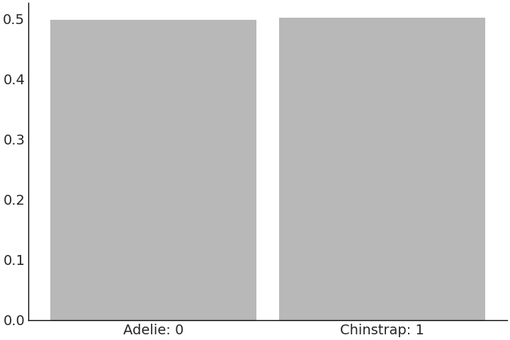
Fig. 3.18 5000 prior predictive samples of class prediction from the model_logistic_penguins_bill_length. This likelihood is discrete, more specifically binary, as opposed to the continuous distribution of mass that was being estimated in earlier models.

After fitting the parameters in our model we can inspect the coefficients using az.summary(.) function (see Table 3.3). While we can read the coefficients they are not as directly interpretable as in a linear regression. We can tell there is some relationship with bill length and species given the positive \(\beta_1\) coefficient whose HDI does not cross zero. We can interpret the decision boundary fairly directly seeing that around 44 mm in bill length is the nominal cutoff for one species to another. Plotting the regression output in Fig. 3.19 is much more intuitive. Here we see the now familiar logistic curve move from 0 on the left to 1 on the right as the classes change, and a decision boundary where one would expect it given the data.

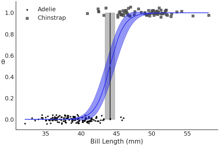
Fig. 3.19 Fitted logistic regression, showing probability curve, observed data points and decision boundary for model_logistic_penguins_bill_length. Looking at just the observed data it seems there is a separation around 45mm bill length for both species, and our model similarly discerned the separation around that value.

Table 3.3 Logistic regression coefficients for model_logistic_penguins_bill_length.

	mean	sd	hdi_3%	hdi_97%
\(\beta_0\)	-46.052	7.073	-58.932	-34.123
\(\beta_1\)	1.045	0.162	0.776	1.347

Let us try something different, we still want to classify penguins but this time using mass as a covariate. Code Block model_logistic_penguins_mass shows a model for that purpose.

Listing 3.22 model_logistic_penguins_mass

mass_obs = penguins.loc[species_filter, "body_mass_g"].values

with pm.Model() as model_logistic_penguins_mass:
    β_0 = pm.Normal("β_0", mu=0, sigma=10)
    β_1 = pm.Normal("β_1", mu=0, sigma=10)

    μ = β_0 + pm.math.dot(mass_obs, β_1)
    θ = pm.Deterministic("θ", pm.math.sigmoid(μ))
    bd = pm.Deterministic("bd", -β_0/β_1)

    yl = pm.Bernoulli("yl", p=θ, observed=species.codes)

    inf_data_logistic_penguins_mass = pm.sample(
        5000, target_accept=.9, return_inferencedata=True)

Table 3.4 Logistic regression coefficients for model_logistic_penguins_mass.

	mean	sd	hdi_3%	hdi_97%
\(\beta_0\)	-1.131	1.317	-3.654	1.268
\(\beta_1\)	0.000	0.000	0.000	0.001

Our tabular summary in Table 3.4 shows that \(\beta_1\) is estimated to be 0 indicating there is not enough information in the mass covariate to separate the two classes. This is not necessarily a bad thing, just the model indicating to us that it does not find discernible difference in mass between these two species. This becomes quite evident once we plot the data and logistic regression fit in Fig. 3.20.

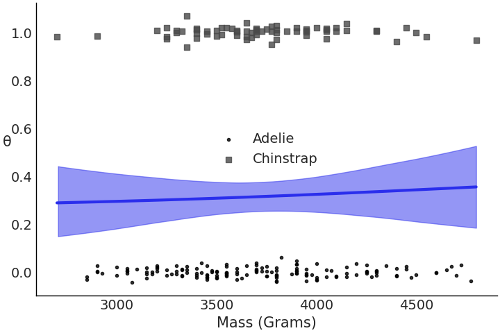
Fig. 3.20 Plot of the observed data and logistic regression for model_logistic_penguins_mass. Unlike Fig. 3.19 the data does not look very separable and our model did discern one as well.

We should not let this lack of relationship discourage us, effective modeling includes a dose of trial an error. This does not mean try random things and hope they work, it instead means that it is ok to use the computational tools to provide you clues to the next step.

Let us now try using both bill length and mass to create a multiple logistic regression in Code Block model_logistic_penguins_bill_length_mass and plot the decision boundary again in Fig. 3.21. This time the axes of the figure are a little bit different. Instead of the probability of class on the Y-axis, we instead have mass. This way we can see the decision boundary between the dependent variables. All these visual checks have been helpful but subjective. We can quantify our fits numerically as well using diagnostics.

Listing 3.23 model_logistic_penguins_bill_length_mass

X = penguins.loc[species_filter, ["bill_length_mm", "body_mass_g"]]

# Add a column of 1s for the intercept
X.insert(0,"Intercept", value=1)
X = X.values

with pm.Model() as model_logistic_penguins_bill_length_mass:
    β = pm.Normal("β", mu=0, sigma=20, shape=3)

    μ = pm.math.dot(X, β)

    θ = pm.Deterministic("θ", pm.math.sigmoid(μ))
    bd = pm.Deterministic("bd", -β[0]/β[2] - β[1]/β[2] * X[:,1])

    yl = pm.Bernoulli("yl", p=θ, observed=species.codes)

    inf_data_logistic_penguins_bill_length_mass = pm.sample(
        1000,
        return_inferencedata=True)

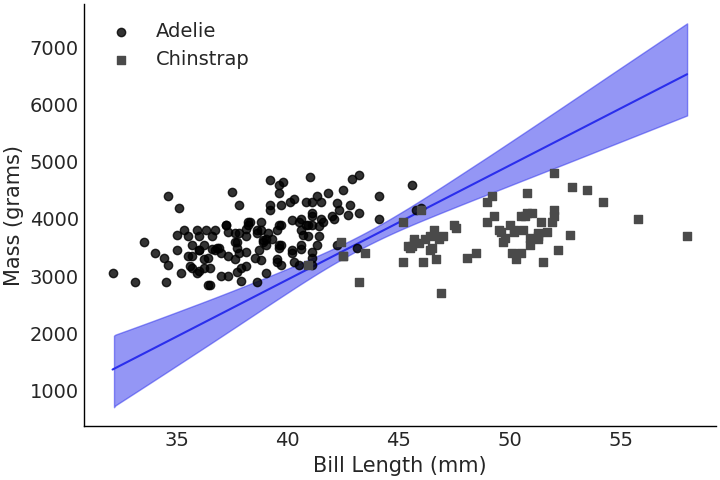
Fig. 3.21 Decision boundary of species class plotted against bill length and mass. We can see that most of the species separability comes from bill length although mass now adds some extra information in regards to class separability as indicated by the slope of the line.

To evaluate the model fit for logistic regressions we can use a separation plot [39], as shown in Code Block separability_plot and Fig. 3.22. A separation plot is a way to assess the calibration of a model with binary observed data. It shows the sorted predictions per class, the idea being that with perfect separation there would be two distinct rectangles. In our case we see that none of our models did a perfect job separating the two species, but the models that included bill length performed much better than the model that included mass only. In general, perfect calibration is not the goal of a Bayesian analysis, nevertheless separation plots (and other calibration assessment methods like LOO-PIT) can help us to compare models and reveal opportunities to improve them.

Listing 3.24 separability_plot

models = {"bill": inf_data_logistic_penguins_bill_length,
          "mass": inf_data_logistic_penguins_mass,
          "mass bill": inf_data_logistic_penguins_bill_length_mass}

_, axes = plt.subplots(3, 1, figsize=(12, 4), sharey=True)
for (label, model), ax in zip(models.items(), axes):
    az.plot_separation(model, "yl", ax=ax, color="C4")
    ax.set_title(label)

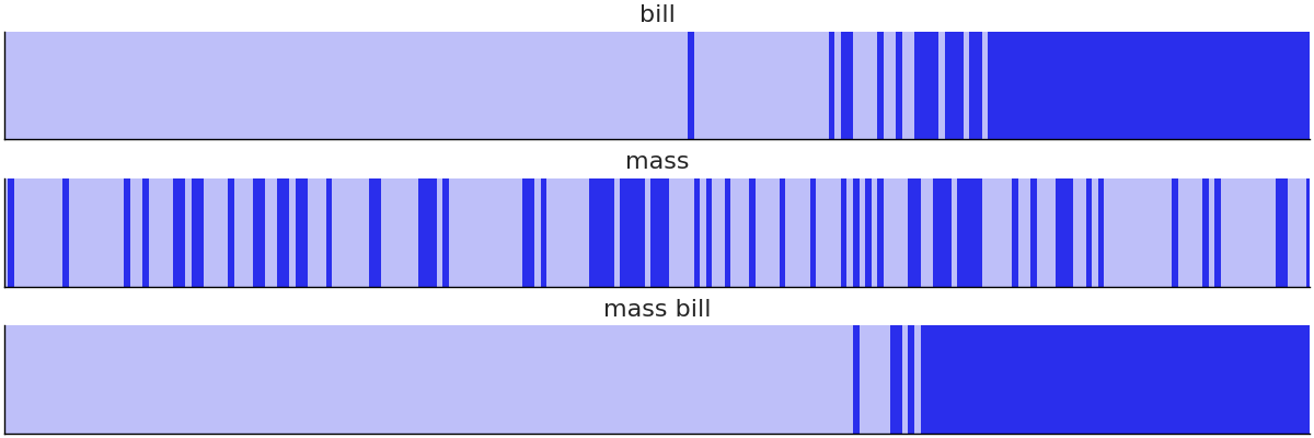
Fig. 3.22 Separation plot of all three penguin models. The light versus dark value indicates the binary class label. In this plot its much more evident that the mass only model does a poor job separating the two species, where are the bill and mass bill models perform better at this task.

We can also use LOO to compare the three models we have just created, the one for the mass, the one for the bill length and the one including both covariates in Code Block penguin_model_loo and Table 3.5. According to LOO the mass only model is the worst at separating the species, the bill length only is the middle candidate model, and the mass and bill length model performed the best. This is unsurprising given what we have seen from the plots, and now we have a numerical confirmation as well.

Listing 3.25 penguin_model_loo

az.compare({"mass":inf_data_logistic_penguins_mass,
            "bill": inf_data_logistic_penguins_bill_length,
            "mass_bill":inf_data_logistic_penguins_bill_length_mass})

Table 3.5 Summary of model comparison. Models are ranked from lowest to highest ELPD values (loo column).

	rank	loo	p_loo	d_loo	weight	se	dse	warning	loo_scale
mass_bill	0	-11.3	1.6	0.0	1.0	3.1	0.0	True	log
bill	1	-27.0	1.7	15.6	0.0	6.2	4.9	True	log
mass	2	-135.8	2.1	124.5	0.0	5.3	5.8	True	log

3.4.3. Interpreting Log Odds

In a logistic regression the slope is telling you the increase in log odds units when x is incremented one unit. Odds most simply are the ratio between the probability of occurrence and probability of no occurrence. For example, in our penguin example if we were to pick a random penguin from Adelie or Chinstrap penguins the probability that we pick an Adelie penguin would be 0.68 as seen in Code Block adelie_prob

Listing 3.26 adelie_prob

# Class counts of each penguin species
counts = penguins["species"].value_counts()
adelie_count = counts["Adelie"],
chinstrap_count = counts["Chinstrap"]
adelie_count / (adelie_count + chinstrap_count)

array([0.68224299])

And for the same event the odds would be

Listing 3.27 adelie_odds

adelie_count / chinstrap_count

array([2.14705882])

Odds are made up of the same components as probability but are transformed in a manner that makes interpreting the ratio of one event occurring from another more straightforward. Stated in odds, if we were to randomly sample from Adelie and Chinstrap penguins we would expect to end up with a ratio of 2.14 more Adelie penguins than Chinstrap penguins as calculated by Code Block adelie_odds.

Using our knowledge of odds we can define the logit. The logit is the natural log of the odds which is the fraction shown in Equation (3.8). We can rewrite the logistic regression in Equation (3.6) in an alternative form of using the logit.

(3.8)\[\log \left(\frac{p}{1-p} \right) = \boldsymbol{X} \beta\]

This alternative formulation lets us interpret the coefficients of logistic regression as the change in log odds. Using this knowledge we can calculate the probability of observing Adelie to Chinstrap penguins given a change in the observed bill length as shown in Code Block logistic_interpretation. Transformations like these are both interesting mathematically, but also very practically useful when discussing statistical results, a topic we will discuss more deeply in Sharing the Results With a Particular Audience).

Listing 3.28 logistic_interpretation

x = 45
β_0 = inf_data_logistic_penguins_bill_length.posterior["β_0"].mean().values
β_1 = inf_data_logistic_penguins_bill_length.posterior["β_1"].mean().values
bill_length = 45

val_1 = β_0 + β_1*bill_length
val_2 = β_0 + β_1*(bill_length+1)

f"""(Class Probability change from 45mm Bill Length to 46mm:
{(special.expit(val_2) -  special.expit(val_1))*100:.0f}%)"""

'Class Probability change from 45mm Bill Length to 46mm: 15%'

3.5. Picking Priors in Regression Models

Now that we are familiar with generalized linear models let us focus on the prior and its effect on posterior estimation. We will be borrowing an example from Regression and Other Stories [40], in particular a study[13] where the relationship between the attractiveness of parents and the percentage of girl births of those parents is explored. In this study researchers estimated the attractiveness of American teenagers on a five-point scale. Eventually many of these subjects had children, of which the ratio of gender per each attractiveness category was calculated, the resulting data points of which are shown in Code Block uninformative_prior_sex_ratio and plotted in Fig. 3.23. In the same code block we also write a model for single variable regression. This time however, focus specifically on how priors and likelihoods should be assessed together and not independently.

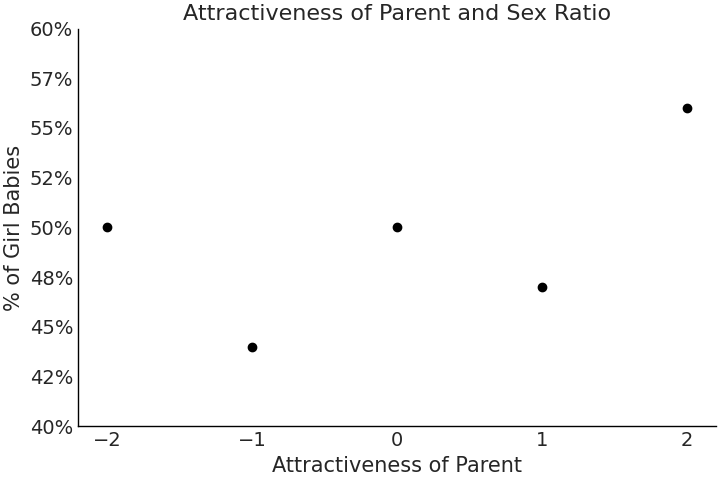
Fig. 3.23 Data on the attractiveness of parents plotted against the gender ratio of their children.

Listing 3.29 uninformative_prior_sex_ratio

x = np.arange(-2, 3, 1)
y = np.asarray([50, 44, 50, 47, 56])

with pm.Model() as model_uninformative_prior_sex_ratio:
    σ = pm.Exponential("σ", .5)
    β_1 = pm.Normal("β_1", 0, 20)
    β_0 = pm.Normal("β_0", 50, 20)

    μ = pm.Deterministic("μ", β_0 + β_1 * x)

    ratio = pm.Normal("ratio", mu=μ, sigma=σ, observed=y)

    prior_predictive_uninformative_prior_sex_ratio = pm.sample_prior_predictive(
        samples=10000
    )
    trace_uninformative_prior_sex_ratio = pm.sample()
    inf_data_uninformative_prior_sex_ratio = az.from_pymc3(
        trace=trace_uninformative_prior_sex_ratio,
        prior=prior_predictive_uninformative_prior_sex_ratio
    )

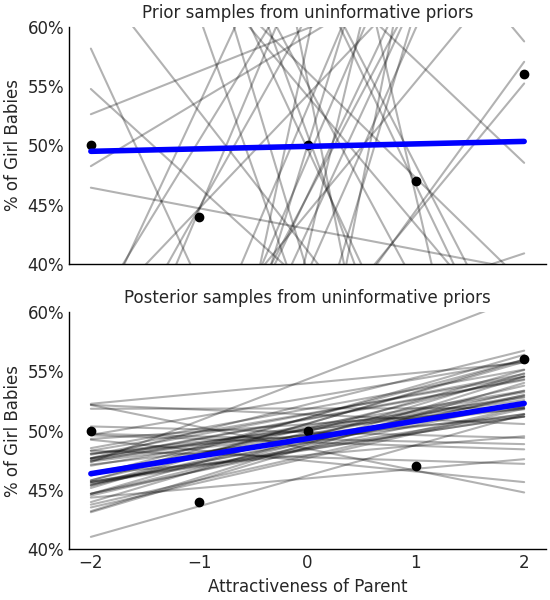
Fig. 3.24 With vague or very wide priors the model shows that large differences in birth ratios are possible for parents rated as attractive. Some of these possible fits are as large as a 20% change which seems implausible as no other study has shown an effect this large on the sex ratio of births.

Nominally we will assume births are equally split between males and females, and that attractiveness has no effect on sex ratio. This translates to setting the mean of the prior for intercept \(\beta_0\) to be 50 and the prior mean for the coefficient \(\beta_1\) to be 0. We also set a wide dispersion to express our lack of knowledge about both the intercept and the effect of attractiveness on sex ratio. This is not a fully uninformative prior, of which we covered in Section A Few Options to Quantify Your Prior Information, however, a very wide prior. Given these choices we can write our model in Code Block uninformative_prior_sex_ratio, run inference, and generate samples to estimate posterior distribution. From the data and model we estimate that the mean of \(\beta_1\) to be 1.4, meaning the least attractive group when compared to the most attractive group the birth ratio will differ by 7.4% on average. In Fig. 3.24 if we include the uncertainty, the ratio can vary by over 20% per unit of attractiveness [10] from a random sample of 50 possible “lines of fit” prior to conditioning the parameters to data.

From a mathematical lens this result is valid. But from the lens of our general knowledge and our understanding of birth sex ratio outside of this studies, these results are suspect. The “natural” sex ratio at birth has been measured to be around 105 boys per 100 girls (ranging from around 103 to 107 boys), which means the sex ratio at birth is 48.5% female, with a standard deviation of 0.5. Moreover, even factors that are more intrinsically tied to human biology do not affect birth ratios to this magnitude, weakening the notion that attractiveness, which is subjective, should have this magnitude of effect. Given this information a change of 8% between two groups would require extraordinary observations.

Let us run our model again but this time set more informative priors shown in Code Block informative_prior_sex_ratio that are consistent with this general knowledge. Plotting our posterior samples the concentration of coefficients is smaller and the plotted posterior lines fall into bounds that are more reasonable when considering possible ratios.

Listing 3.30 informative_prior_sex_ratio

with pm.Model() as model_informative_prior_sex_ratio:
    σ = pm.Exponential("σ", .5)

    # Note the now more informative priors
    β_1 = pm.Normal("β_1", 0, .5)
    β_0 = pm.Normal("β_0", 48.5, .5)

    μ = pm.Deterministic("μ", β_0 + β_1 * x)
    ratio = pm.Normal("ratio", mu=μ, sigma=σ, observed=y)

    prior_predictive_informative_prior_sex_ratio = pm.sample_prior_predictive(
        samples=10000
    )
    trace_informative_prior_sex_ratio = pm.sample()
    inf_data_informative_prior_sex_ratio = az.from_pymc3(
        trace=trace_informative_prior_sex_ratio,
        prior=prior_predictive_informative_prior_sex_ratio)

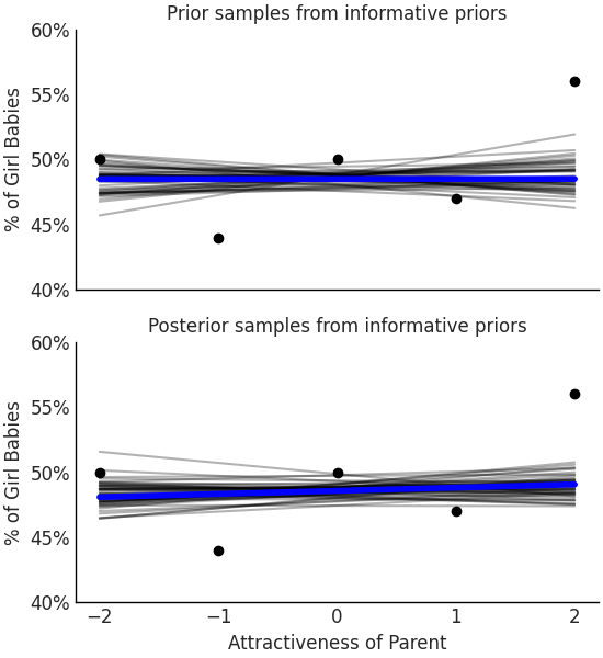
Fig. 3.25 With priors informed from other papers and domain expertise the mean posterior hardly changes across attractiveness ratio indicating that if there is a belief there is an effect on birth ratio from the parents attractiveness more data should be collected to showcase the effect.

This time we see that estimated effect of attractiveness on gender is negligible, there simply was not enough information to affect the posterior. As we mentioned in Section A Few Options to Quantify Your Prior Information choosing a prior is both a burden and a blessing. Regardless of which you believe it is, it is important to use this statistical tool with an explainable and principled choice.

3.6. Exercises

E1. Comparisons are part of everyday life. What is something you compare on a daily basis and answer the following question:

• What is the numerical quantification you use for comparison?

• How do you decide on the logical groupings for observations? For example in the penguin model we use species or sex

• What point estimate would you use to compare them?

E2. Referring to Model penguin_mass complete the following tasks.

1. Compute the values of Monte Carlo Standard Error Mean using az.summary. Given the computed values which of the following reported values of \(\mu\) would not be well supported as a point estimate? 3707.235, 3707.2, or 3707.

2. Plot the ESS and MCSE per quantiles and describe the results.

3. Resample the model using a low number of draws until you get bad values of \(\hat R\), and ESS

4. Report the HDI 50% numerically and using az.plot_posterior

E3. In your own words explain how regression can be used to do the following:

1. Covariate estimation

2. Prediction

3. Counterfactual analysis

Explain how they are different, the steps to perform each, and situations where they would be useful. Use the penguin example or come up with your own.

E4. In Code Block flipper_centering and Code Block tfp_penguins_centered_predictor we centered the flipper length covariate. Refit the model, but instead of centering, subtract the minimum observed flipped length. Compare the posterior estimates of the slope and intercept parameters of the centered model. What is different, what is the same. How does the interpretation of this model change when compared to the centered model?

E5. Translate the following primitives from PyMC3 to TFP. Assume the model name is pymc_model

1. pm.StudentT("x", 0, 10, 20)

2. pm.sample(chains=2)

Hint: write the model and inference first in PyMC3, and find the similar primitives in TFP using the code shown in this chapter.

E6. PyMC3 and TFP use different argument names for their distribution parameterizations. For example in PyMC3 the Uniform Distribution is parameterized as pm.Uniform.dist(lower=, upper=) whereas in TFP it is tfd.Uniform(low=, high=). Use the online documentation to identify the difference in argument names for the following distributions.

1. Normal

2. Poisson

3. Beta

4. Binomial

5. Gumbel

E7. A common modeling technique for parameterizing Bayesian multiple regressions is to assign a wide prior to the intercept, and assign more informative prior to the slope coefficients. Try modifying the model_logistic_penguins_bill_length_mass model in Code Block model_logistic_penguins_bill_length_mass. Do you get better inference results? Note that there are divergences with the original parameterization.

E8. In linear regression models we have two terms. The mean linear function and the noise term. Write down these two terms in mathematical notation, referring to the equations in this chapter for guidance. Explain in your own words what the purpose of these two parts of regression are. In particular why are they useful when there is random noise in any part of the data generating or data collection process.

E9. Simulate the data using the formula y = 10 + 2x + \(\mathcal{N}(0, 5)\) with integer covariate x generated np.linspace(-10, 20, 100). Fit a linear model of the form \(b_0 + b_1*X + \sigma\). Use a Normal distribution for the likelihood and covariate priors and a Half Student’s T prior for the noise term as needed. Recover the parameters verifying your results using both a posterior plot and a forest plot.

E10. Generate diagnostics for the model in Code Block non_centered_regression to verify the results shown in the chapter can be trusted. Use a combination of visual and numerical diagnostics.

E11. Refit the model in Code Block non_centered_regression on Gentoo penguins and Chinstrap penguins. How are the posteriors different from each other? How are they different from the Adelie posterior estimation? What inferences can you make about the relationship between flipper length and mass for these other species of penguins? What does the change in \(\sigma\) tell you about the ability of flipper length to estimate mass?

M12. Using the model in Code Block tfp_flipper_bill_sex_counterfactuals run a counterfactual analysis for female penguin flipper length with mean flipper length and a bill length of 20mm. Plot a kernel density estimate of the posterior predictive samples.

M13. Duplicate the flipper length covariate in Code Block non_centered_regression by adding a \(\beta_2\) coefficient and rerun the model. What do diagnostics such as ESS and rhat indicate about this model with a duplicated coefficient?

M14. Translate the PyMC3 model in Code Block non_centered_regression into Tensorflow Probability. List three of the syntax differences.

M15. Translate the TFP model in Code Block tfp_penguins_centered_predictor into PyMC3. List three of the syntax differences.

M16. Use a logistic regression with increasing number of covariates to reproduce the prior predictive distributions in Fig. 2.3. Explain why its the case that a logistic regression with many covariates generate a prior response with extreme values.

H17. Translate the PyMC3 model in Code Block model_logistic_penguins_bill_length_mass into TFP to classify Adelie and Chinstrap penguins. Reuse the same model to classify Chinstrap and Gentoo penguins. Compare the coefficients, how do they differ?

H18. In Code Block penguin_mass our model allowed for negative values mass. Change the model so negative values are no longer possible. Run a prior predictive check to verify that your change was effective. Perform MCMC sampling and plot the posterior. Has the posterior changed from the original model? Given the results why would you choose one model over the other and why?

H19. The Palmer Penguin dataset includes additional data for the observed penguins such as island and bill depth. Include these covariates into the linear regression model defined in Code Block non_centered_regression in two parts, first adding bill depth, and then adding the island covariates. Do these covariates help estimate Adelie mass more precisely? Justify your answer using the parameter estimates and model comparison tools.

H20. Similar the exercise 2H19, see if adding bill depth or island covariates to the penguin logistic regression help classify Adelie and Gentoo penguins more precisely. Justify if the additional covariates helped using the numerical and visual tools shown in this chapter.

---

[1]

You can find more information in the TensorFlow tutorials and documentations. For example, https://www.tensorflow.org/probability/examples/JointDistributionAutoBatched_A_Gentle_Tutorial and https://www.tensorflow.org/probability/examples/Modeling_with_JointDistribution.

[2]

tfd.Sample and tfd.Independent are distribution constructors that takes other distributions as input and return a new distribution. There are other meta distribution but with different purposes like tfd.Mixture, tfd.TransformedDistribution, and tfd.JointDistribution. A more comprehensive introduction to tfp.distributions can be found in https://www.tensorflow.org/probability/examples/TensorFlow_Distributions_Tutorial

[3]

https://mc-stan.org/docs/2_23/reference-manual/hmc-algorithm-parameters.html#automatic-parameter-tuning

[4]

If wanted exactly the same model we could specify the priors in Bambi, not shown here. For our purposes however, the models are “close enough”.

[5]

You can also parse the design matrix differently so that covariates represents the contrast between 2 categories within a column.

[6]

Maybe because collecting more data is expensive or difficult or even impossible

[7]

Unless we are talking about large systems like rain forests, where the presence of plants actually have an impact in the weather. Nature can be hard to grasp with simple statements.

[8]

Traditionally people apply functions like \(\phi\) to the left side of Equation (3.5), and call them link functions. We instead prefer to apply them to the right-hand side and then to avoid confusion we use term inverse link function.

[9]

Usually in the traditional Generalized Linear Models Literature, the likelihood of the observation need to be from the Exponential family, but being Bayesian we are actually not restricted by that and can use any likelihood that can be parameterized by the expected value.

[10]

Estimate shown in corresponding notebook.