Code 2: Exploratory Analysis of Bayesian Models

This is a reference notebook for the book Bayesian Modeling and Computation in Python

The textbook is not needed to use or run this code, though the context and explanation is missing from this notebook.

If you’d like a copy it’s available from the CRC Press or from Amazon. ``

%matplotlib inline
import arviz as az
import matplotlib.pyplot as plt
import numpy as np
import pymc3 as pm
from scipy import stats
import theano.tensor as tt

az.style.use("arviz-grayscale")
plt.rcParams['figure.dpi'] = 300
np.random.seed(5201)

Understanding Your Assumptions

Figure 2.2

half_length = 3.66  # meters
penalty_point = 11  # meters
def Phi(x):
    """Calculates the standard normal cumulative distribution function."""
    return 0.5 + 0.5 * tt.erf(x / tt.sqrt(2.0))


ppss = []
sigmas_deg = [5, 20, 60]
sigmas_rad = np.deg2rad(sigmas_deg)
for sigma in sigmas_rad:
    with pm.Model() as model:
        σ = pm.HalfNormal("σ", sigma)
        α = pm.Normal("α", 0, σ)
        p_goal = pm.Deterministic("p_goal", 2 * Phi(tt.arctan(half_length / penalty_point) / σ) - 1)
        pps = pm.sample_prior_predictive(250)
        ppss.append(pps)

fig, axes = plt.subplots(1, 3, subplot_kw=dict(projection="polar"), figsize=(10, 4))

max_angle = np.arctan(half_length/penalty_point)

for sigma, pps, ax in zip(sigmas_deg, ppss, axes):
    cutoff = pps["p_goal"] > 0.1
    cax = ax.scatter(pps["α"][cutoff], np.ones_like(pps["α"][cutoff]), c=pps["p_goal"][cutoff],
               marker=".", cmap="viridis_r", vmin=0.1)
    ax.fill_between(np.linspace(-max_angle, max_angle, 100), 0, 1.01, alpha=0.25)
    ax.set_yticks([])
    ax.set_title(f"$\sigma = \mathcal{{HN}}({sigma})$")
    ax.plot(0,0, 'o')
fig.colorbar(cax, extend="min", ticks=[1, 0.5, 0.1], shrink=0.7, aspect=40)

plt.savefig("img/chp02/prior_predictive_distributions_00.png", bbox_inches="tight")

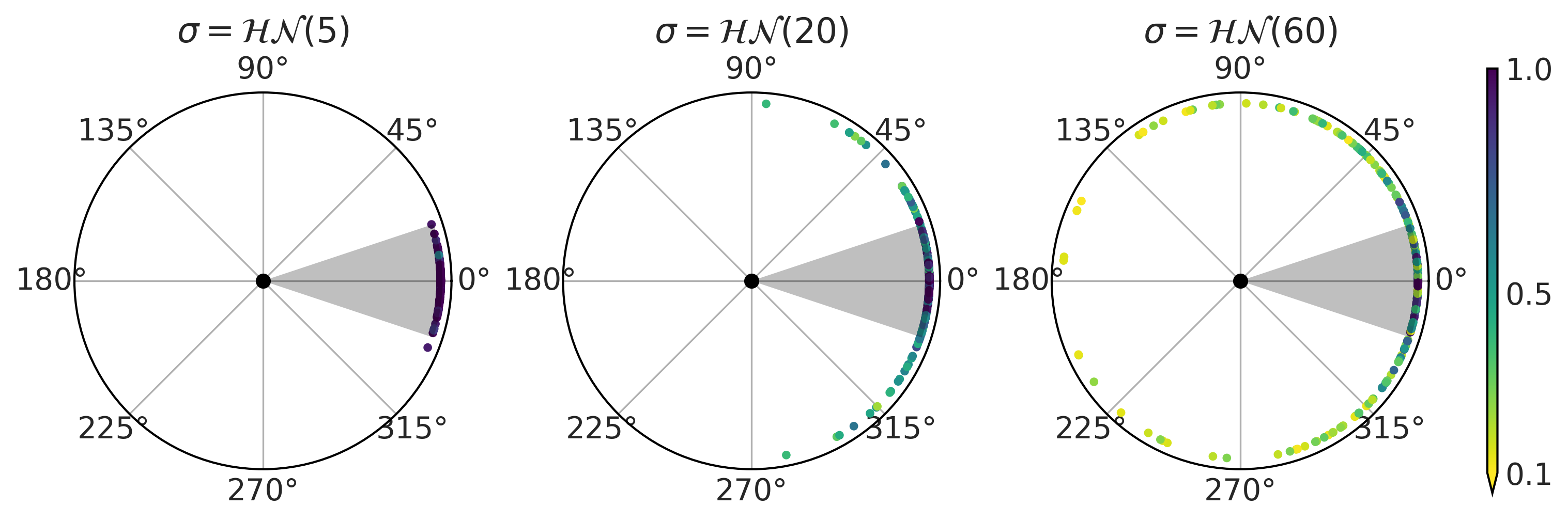
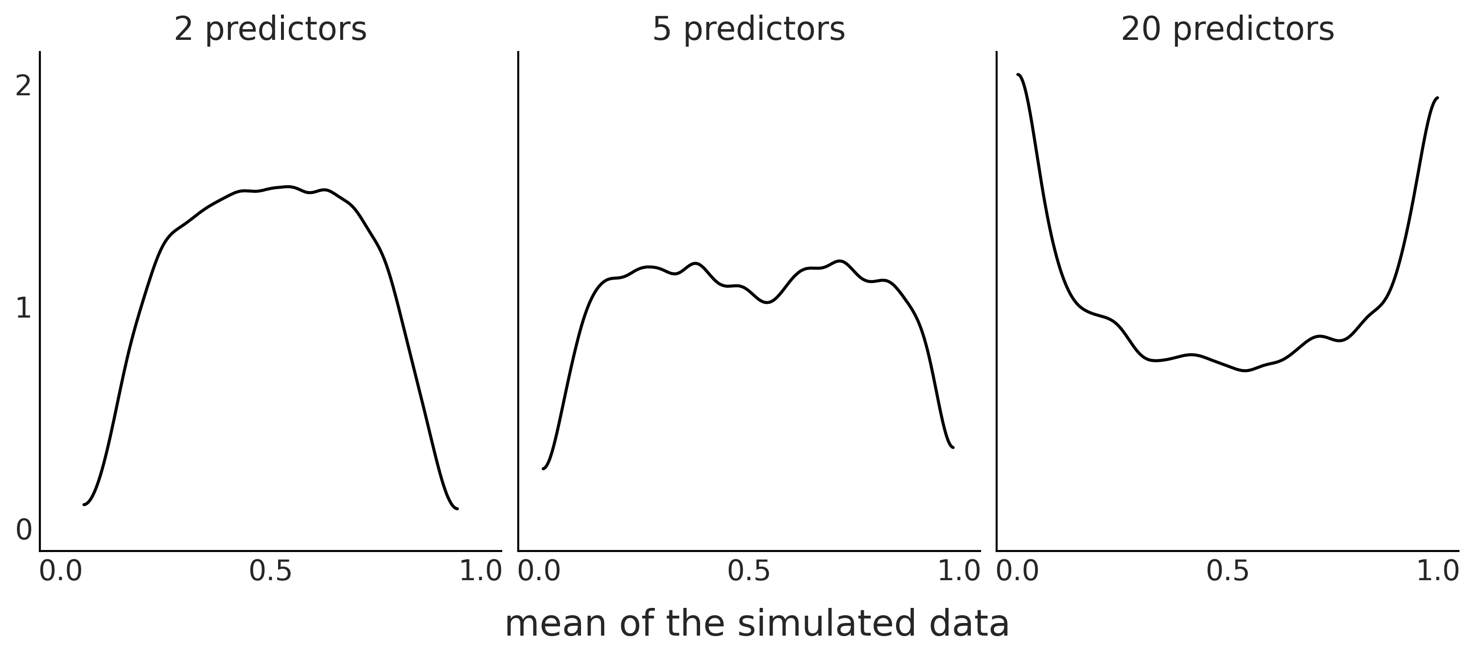
Figure 2.3

from scipy.special import expit
fig, axes = plt.subplots(1, 3, figsize=(10, 4), sharex=True,  sharey=True)
axes = np.ravel(axes)

for dim, ax in zip([2, 5, 20], axes):
    β = np.random.normal(0, 1, size=(10000, dim))
    X = np.random.binomial(n=1, p=0.75, size=(dim, 500))
    az.plot_kde(expit(β @ X).mean(1), ax=ax)
    ax.set_title(f"{dim} predictors")
    ax.set_xticks([0, 0.5, 1])
    ax.set_yticks([0, 1, 2])

fig.text(0.34, -0.075, size=18, s="mean of the simulated data")
plt.savefig("img/chp02/prior_predictive_distributions_01.png", bbox_inches="tight")

Understanding Your Predictions

Figure 2.4

Y = stats.bernoulli(0.7).rvs(100)
with pm.Model() as model:
    θ = pm.Beta("θ", 1, 1)
    y_obs = pm.Binomial("y_obs",n=1, p=θ, observed=Y)
    trace_b = pm.sample(1000)

<ipython-input-6-2e8727eee630>:5: FutureWarning: In v4.0, pm.sample will return an `arviz.InferenceData` object instead of a `MultiTrace` by default. You can pass return_inferencedata=True or return_inferencedata=False to be safe and silence this warning.
  trace_b = pm.sample(1000)
Auto-assigning NUTS sampler...
Initializing NUTS using jitter+adapt_diag...
Multiprocess sampling (4 chains in 4 jobs)
NUTS: [θ]

100.00% [8000/8000 00:01<00:00 Sampling 4 chains, 0 divergences]

Sampling 4 chains for 1_000 tune and 1_000 draw iterations (4_000 + 4_000 draws total) took 2 seconds.

pred_dist = pm.sample_posterior_predictive(trace_b, 1000, model=model)["y_obs"]

/u/32/martino5/unix/anaconda3/envs/pymcv3/lib/python3.9/site-packages/pymc3/sampling.py:1689: UserWarning: samples parameter is smaller than nchains times ndraws, some draws and/or chains may not be represented in the returned posterior predictive sample
  warnings.warn(

100.00% [1000/1000 00:00<00:00]

_, ax = plt.subplots(1, 2, figsize=(12, 4), constrained_layout=True)

az.plot_dist(pred_dist.sum(1),
             hist_kwargs={"color":"C2"}, ax=ax[0])
ax[0].axvline(Y.sum(), color="C4", lw=2.5);
ax[0].axvline(pred_dist.sum(1).mean(), color="k", ls="--")
ax[0].set_yticks([])
ax[0].set_xlabel("number of success")

pps_ = pred_dist.mean(1)
ax[1].plot((np.zeros_like(pps_), np.ones_like(pps_)), (1-pps_, pps_), 'C1', alpha=0.01)

ax[1].plot((0, 1), (1-Y.mean(), Y.mean()), 'C4', lw=2.5)
ax[1].plot((0, 1), (1-pps_.mean(), pps_.mean()), 'k--')
ax[1].set_xticks((0,1))
ax[1].set_xlabel("observed values")
ax[1].set_ylabel("probability")
plt.savefig("img/chp02/posterior_predictive_check.png")

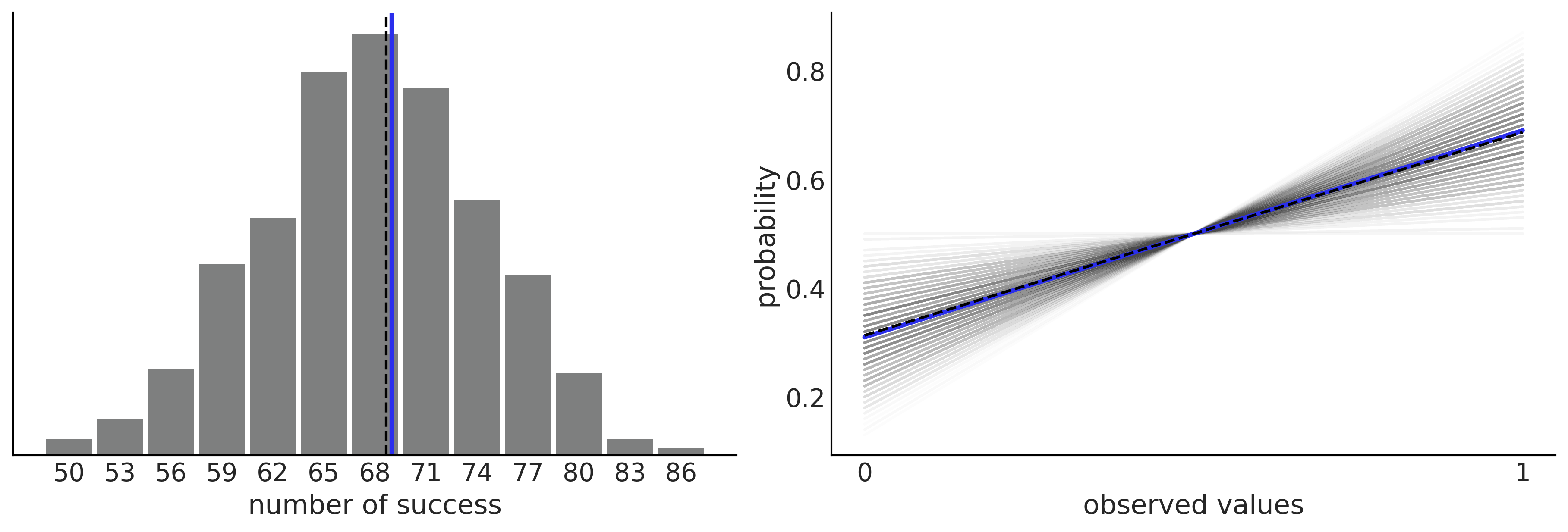
Figure 2.5

idata = az.from_dict(posterior_predictive={"y":pred_dist.reshape(2, 500, 100)}, observed_data={"y":Y})

_, ax = plt.subplots(1, 2, figsize=(10, 4))
az.plot_bpv(idata, kind="p_value", ax=ax[0])
ax[0].legend([f"bpv={(Y.mean() > pred_dist.mean(1)).mean():.2f}"], handlelength=0)
az.plot_bpv(idata, kind="u_value", ax=ax[1])
ax[1].set_yticks([])
ax[1].set_xticks([0., 0.5, 1.])
plt.savefig("img/chp02/posterior_predictive_check_pu_values.png")

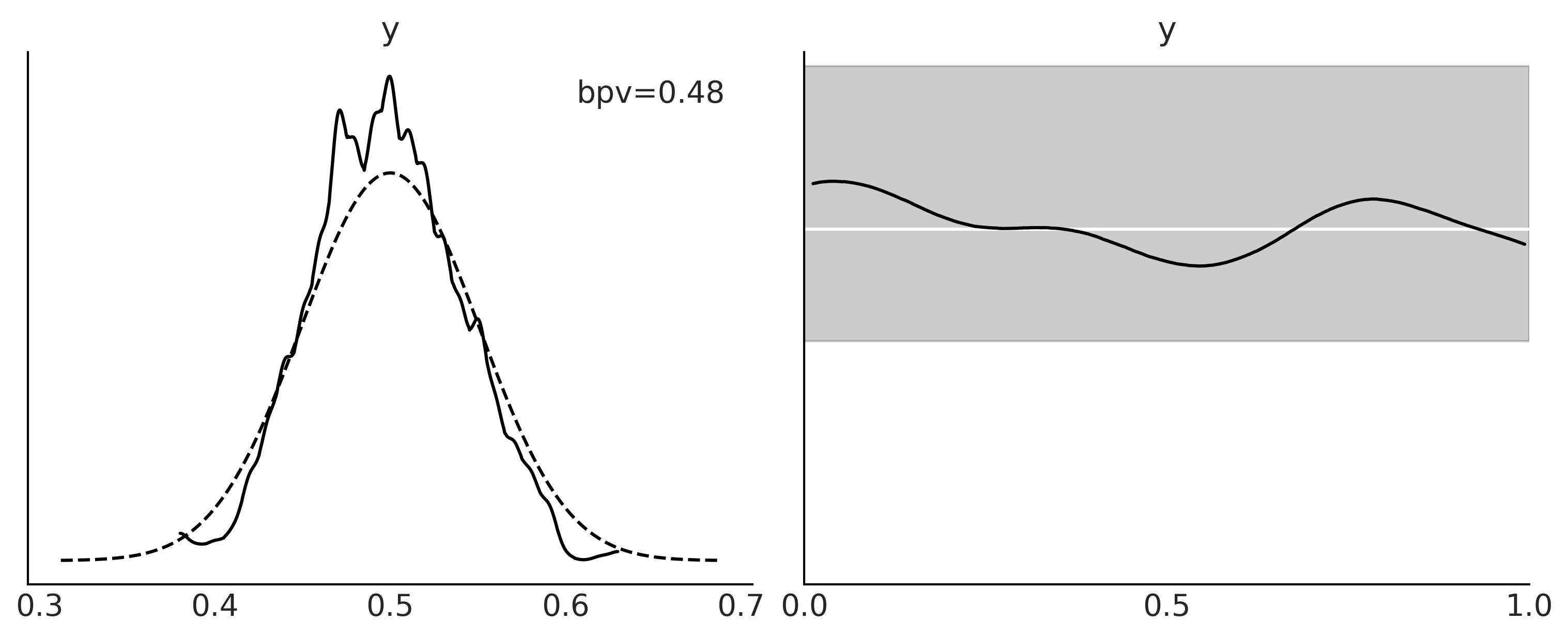
Figure 2.6

_, ax = plt.subplots(1, 2, figsize=(10, 4))
az.plot_bpv(idata, kind="t_stat", t_stat="mean", ax=ax[0])
ax[0].set_title("mean")
az.plot_bpv(idata, kind="t_stat", t_stat="std", ax=ax[1])
ax[1].set_title("standard deviation")
ax[1].set_xticks([0.32, 0.41, 0.5])
plt.savefig("img/chp02/posterior_predictive_check_tstat.png")

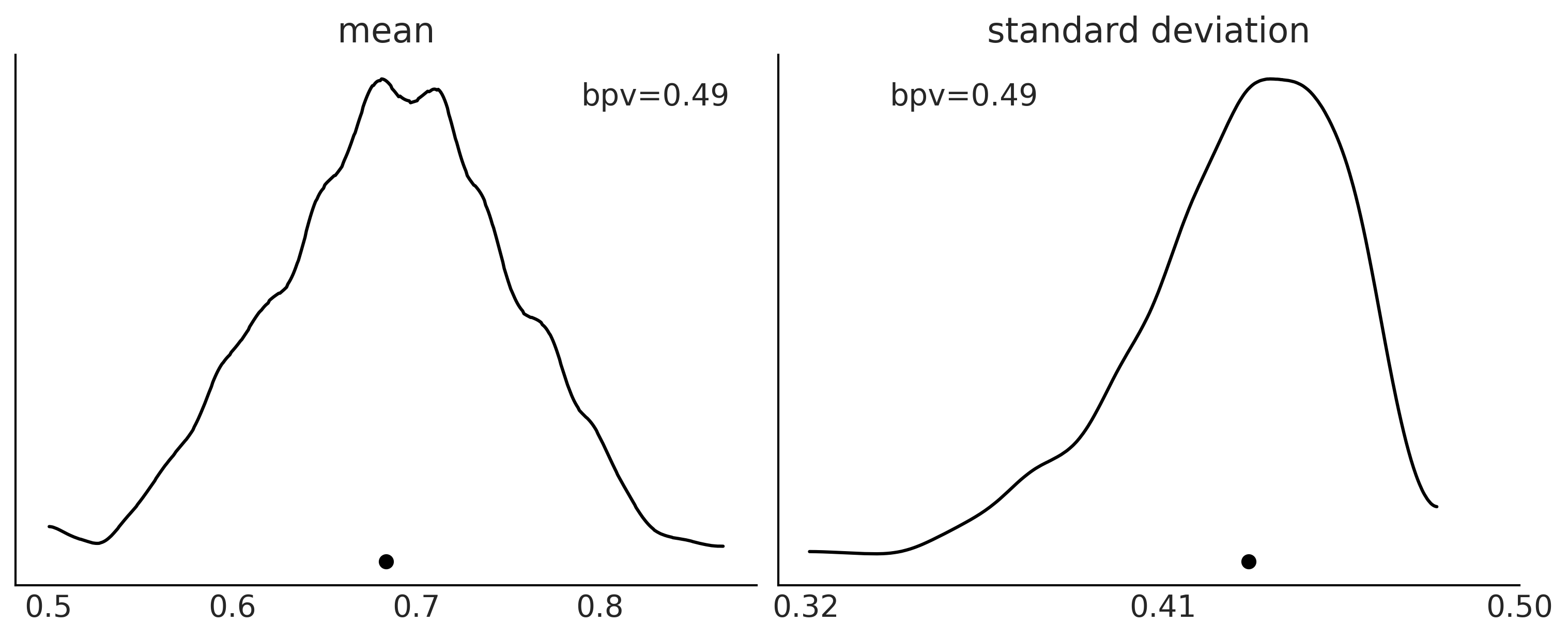
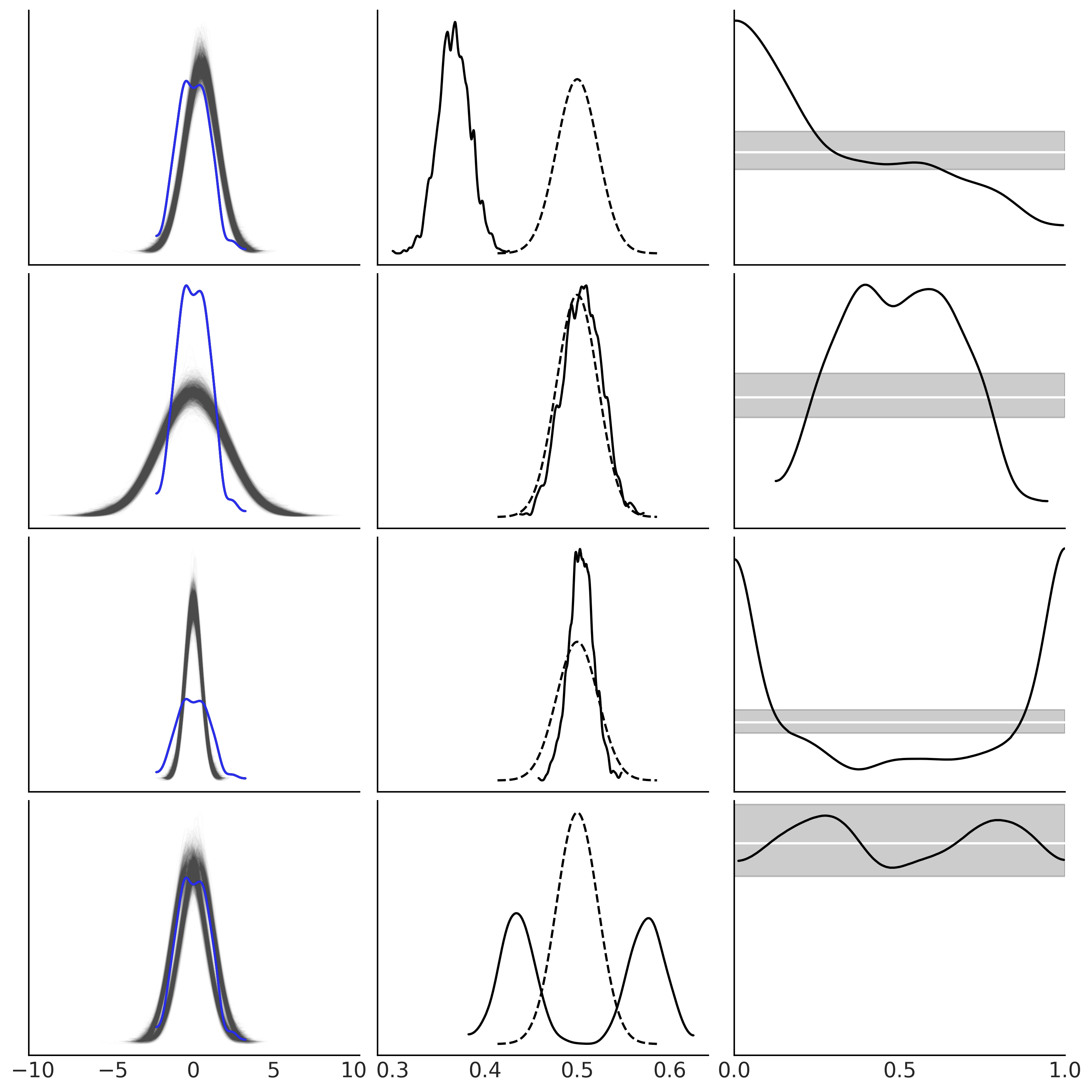
Figure 2.7

n_obs = 500
samples = 2000
y_obs = np.random.normal(0, 1, size=n_obs)

idata1 = az.from_dict(posterior_predictive={"y":np.random.normal(0.5, 1, size=(1, samples, n_obs))},
                      observed_data={"y":y_obs})

idata2 = az.from_dict(posterior_predictive={"y":np.random.normal(0, 2, size=(1, samples, n_obs))},
                      observed_data={"y":y_obs})

idata3 = az.from_dict(posterior_predictive={"y":np.random.normal(0, 0.5, size=(1, samples,n_obs))},
                      observed_data={"y":y_obs})

idata4 = az.from_dict(posterior_predictive={"y":np.concatenate(
                                                [np.random.normal(-0.25, 1, size=(1, samples//2, n_obs)),
                                                 np.random.normal(0.25, 1, size=(1, samples//2, n_obs))]
                                                                )},
                      observed_data={"y":y_obs})

idatas = [idata1,
          idata2,
          idata3,
          idata4,
]

_, axes = plt.subplots(len(idatas), 3, figsize=(10, 10), sharex="col")

for idata, ax in zip(idatas, axes):
    az.plot_ppc(idata, ax=ax[0], color="C1", alpha=0.01, mean=False, legend=False)
    az.plot_kde(idata.observed_data["y"], ax=ax[0], plot_kwargs={"color":"C4", "zorder":3})
    ax[0].set_xlabel("")
    az.plot_bpv(idata, kind="p_value", ax=ax[1])
    az.plot_bpv(idata, kind="u_value", ax=ax[2])
    ax[2].set_yticks([])
    ax[2].set_xticks([0., 0.5, 1.])
    for ax_ in ax:
        ax_.set_title("")

plt.savefig("img/chp02/posterior_predictive_many_examples.png")

Diagnosing Numerical Inference

Code 2.1

np.random.seed(5201)

good_chains = stats.beta.rvs(2, 5,size=(2, 2000))
bad_chains0 = np.random.normal(np.sort(good_chains, axis=None), 0.05,
                               size=4000).reshape(2, -1)

bad_chains1 = good_chains.copy()
for i in np.random.randint(1900, size=4):
    bad_chains1[i%2:,i:i+100] = np.random.beta(i, 950, size=100)

chains = {"good_chains":good_chains,
          "bad_chains0":bad_chains0,
          "bad_chains1":bad_chains1}

Code 2.2

az.ess(chains)

<xarray.Dataset>
Dimensions:      ()
Data variables:
    good_chains  float64 4.389e+03
    bad_chains0  float64 2.436
    bad_chains1  float64 111.1

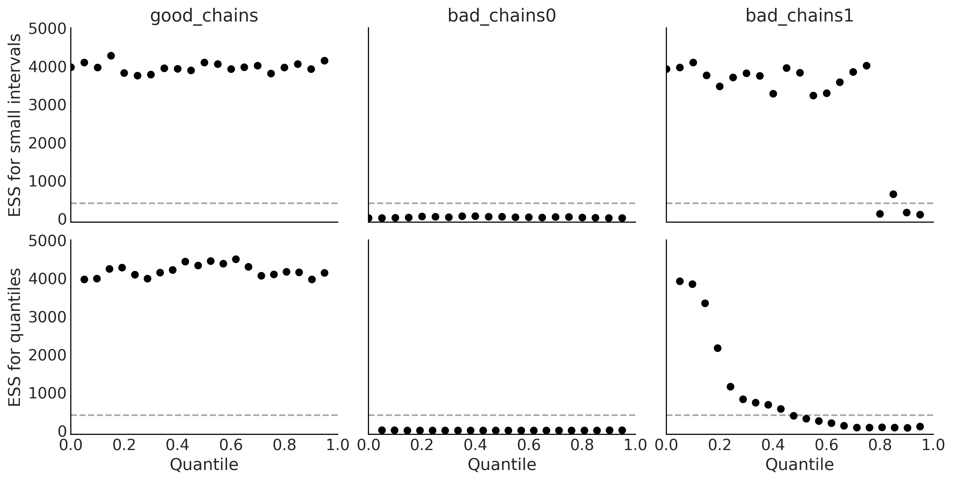
Code 2.3 and Figure 2.8

_, axes = plt.subplots(2, 3, figsize=(12, 6), sharey=True, sharex=True)
az.plot_ess(chains, kind="local", ax=axes[0])
az.plot_ess(chains, kind="quantile", ax=axes[1])

for ax_ in axes[0]:
    ax_.set_xlabel("")
for ax_ in axes[1]:
    ax_.set_title("")

for ax_ in axes[:,1:].ravel():
    ax_.set_ylabel("")
plt.ylim(-100, 5000)
plt.savefig("img/chp02/plot_ess.png")

Code 2.4

az.rhat(chains)

<xarray.Dataset>
Dimensions:      ()
Data variables:
    good_chains  float64 1.0
    bad_chains0  float64 2.408
    bad_chains1  float64 1.033

Code 2.5

az.mcse(chains)

<xarray.Dataset>
Dimensions:      ()
Data variables:
    good_chains  float64 0.002381
    bad_chains0  float64 0.1077
    bad_chains1  float64 0.01781

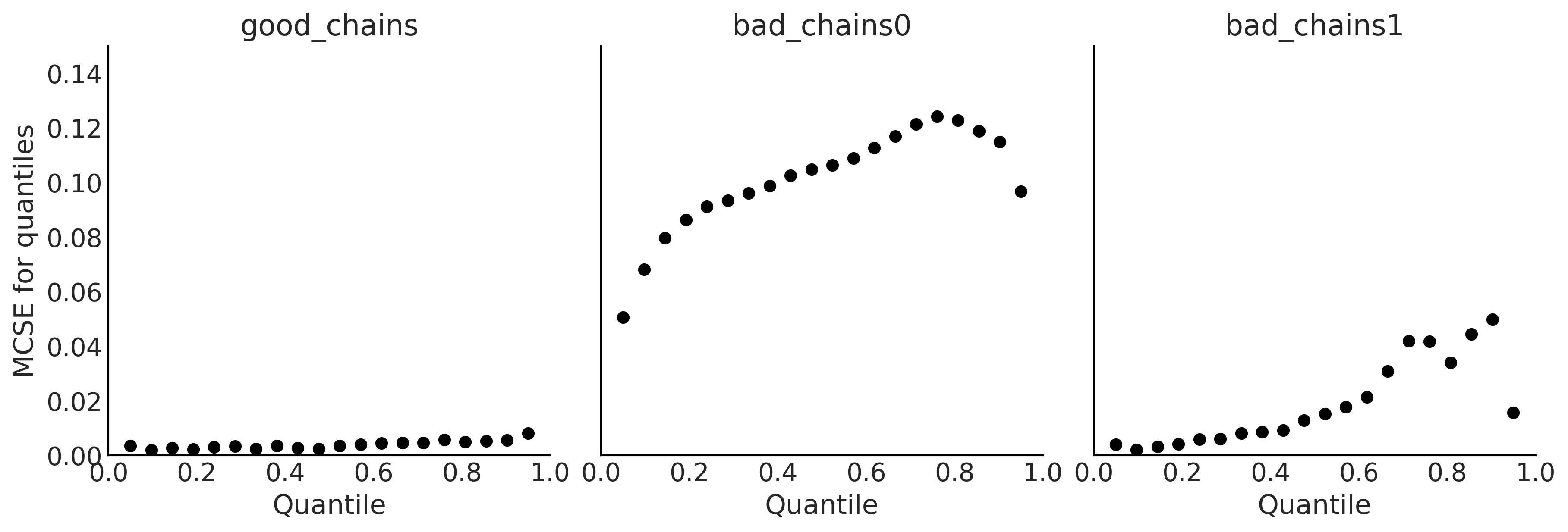
Code 2.6 and Figure 2.9

_, axes = plt.subplots(1, 3, figsize=(12, 4), sharey=True)
az.plot_mcse(chains, ax=axes)
for ax_ in axes[1:]:
    ax_.set_ylabel("")
    ax_.set_ylim(0, 0.15)

plt.savefig("img/chp02/plot_mcse.png")

Code 2.7

az.summary(chains, kind="diagnostics")

	mcse_mean	mcse_sd	ess_bulk	ess_tail	r_hat
good_chains	0.002	0.002	4389.0	3966.0	1.00
bad_chains0	0.108	0.088	2.0	11.0	2.41
bad_chains1	0.018	0.013	111.0	105.0	1.03

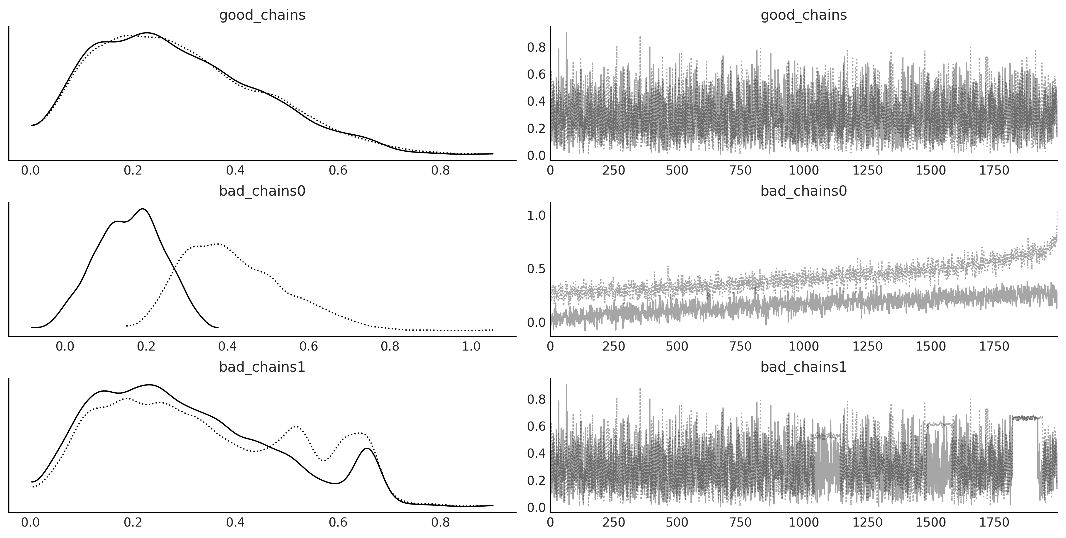
Code 2.8 and Figure 2.10

az.plot_trace(chains)
plt.savefig("img/chp02/trace_plots.png")

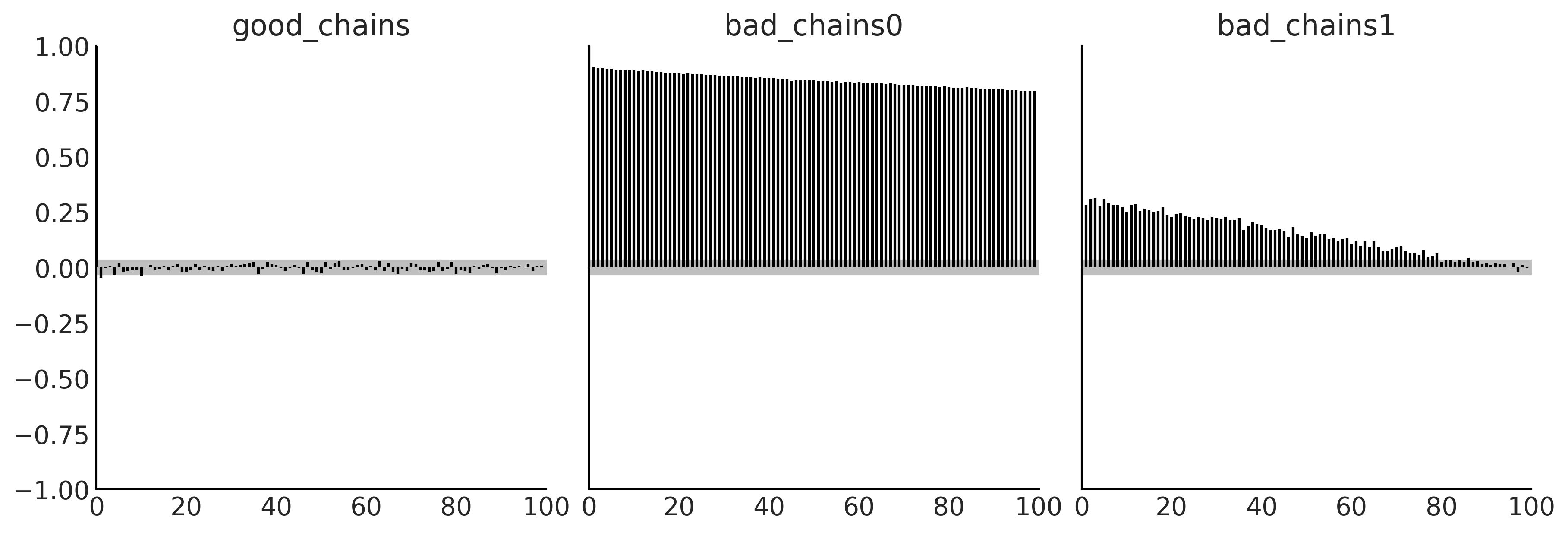
Code 2.9 and Figure 2.11

az.plot_autocorr(chains, combined=True, figsize=(12, 4))
plt.savefig('img/chp02/autocorrelation_plot.png')

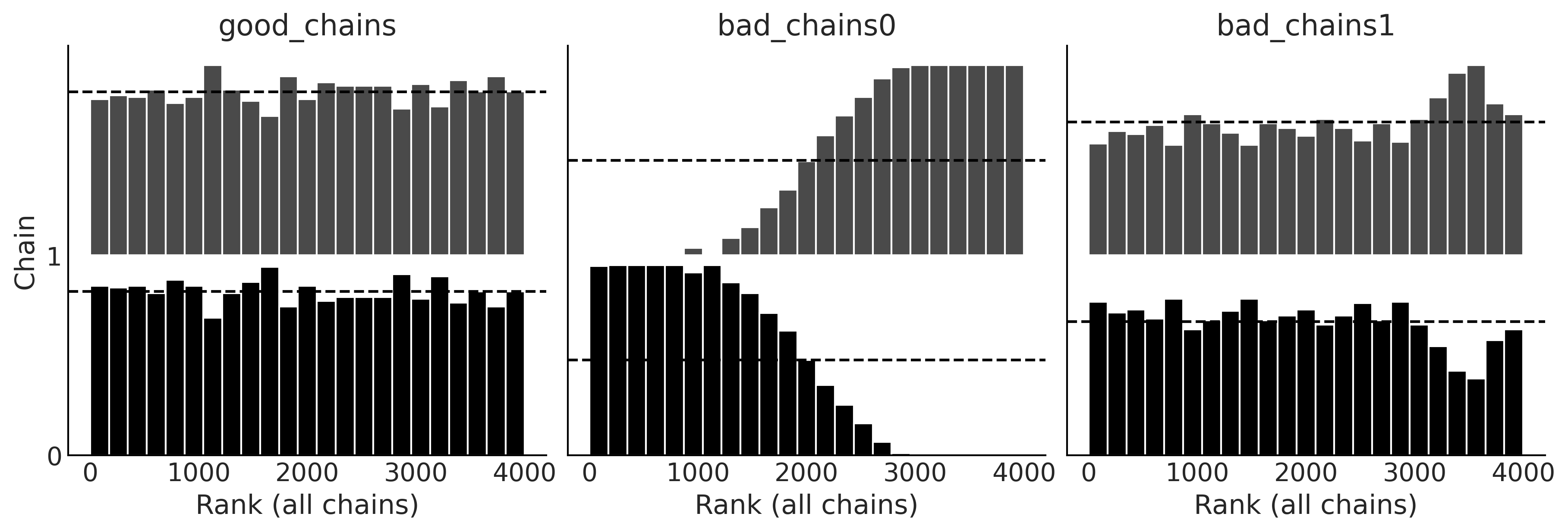
Code 2.10 and Figure 2.12

_, axes = plt.subplots(1, 3, figsize=(12, 4))
az.plot_rank(chains, kind="bars", ax=axes)
for ax_ in axes[1:]:
    ax_.set_ylabel("")
    ax_.set_yticks([])

plt.savefig('img/chp02/rank_plot_bars.png')

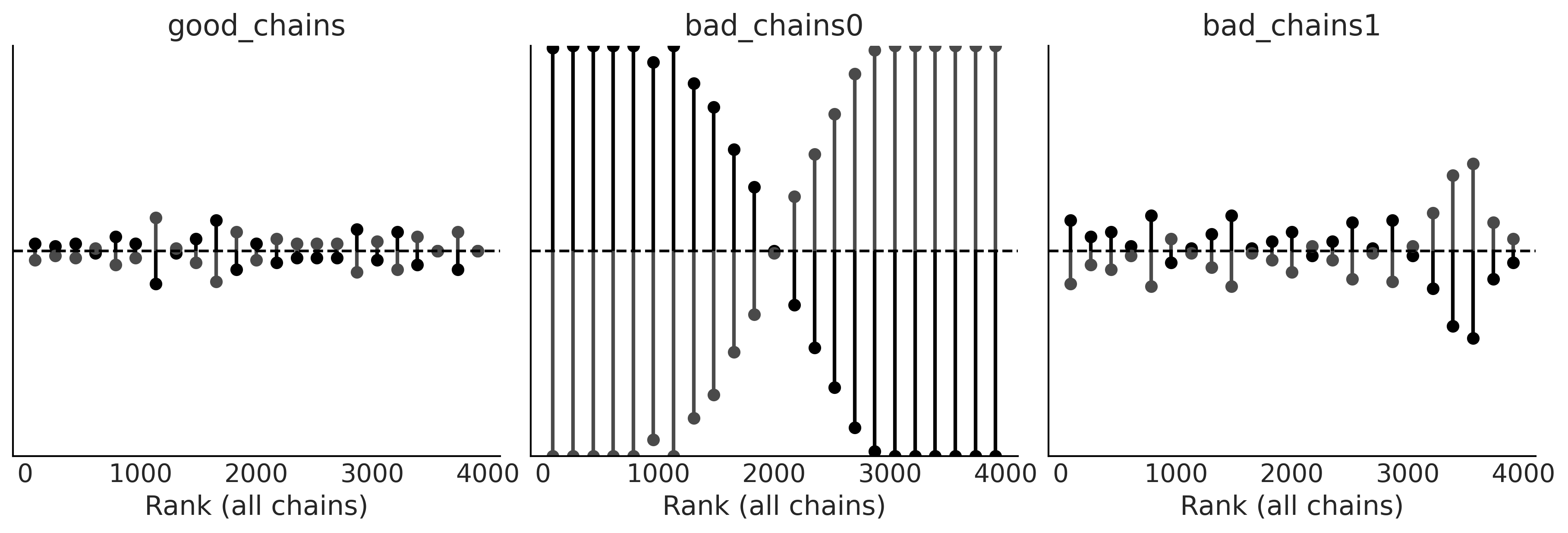
Code 2.11 and Figure 2.13

az.plot_rank(chains, kind="vlines", figsize=(12, 4))
plt.savefig('img/chp02/rank_plot_vlines.png')

Code 2.12, 2.13, and 2.14

with pm.Model() as model_0:
    θ1 = pm.Normal("θ1", 0, 1, testval=0.1)
    θ2 = pm.Uniform("θ2", -θ1, θ1)
    idata_0 = pm.sample(return_inferencedata=True)

with pm.Model() as model_1:
    θ1 = pm.HalfNormal("θ1", 1 / (2/np.pi)**0.5)
    θ2 = pm.Uniform("θ2", -θ1, θ1)
    idata_1 = pm.sample(return_inferencedata=True)

with pm.Model() as model_1bis:
    θ1 = pm.HalfNormal("θ1", 1 / (2/np.pi)**0.5)
    θ2 = pm.Uniform("θ2", -θ1, θ1)
    idata_1bis = pm.sample(return_inferencedata=True, target_accept=0.95)

idatas = [idata_0, idata_1, idata_1bis]

Auto-assigning NUTS sampler...
Initializing NUTS using jitter+adapt_diag...
Multiprocess sampling (4 chains in 4 jobs)
NUTS: [θ2, θ1]

100.00% [8000/8000 00:01<00:00 Sampling 4 chains, 2,300 divergences]

Sampling 4 chains for 1_000 tune and 1_000 draw iterations (4_000 + 4_000 draws total) took 2 seconds.
There were 503 divergences after tuning. Increase `target_accept` or reparameterize.
There were 579 divergences after tuning. Increase `target_accept` or reparameterize.
There were 614 divergences after tuning. Increase `target_accept` or reparameterize.
There were 604 divergences after tuning. Increase `target_accept` or reparameterize.
The number of effective samples is smaller than 25% for some parameters.
Auto-assigning NUTS sampler...
Initializing NUTS using jitter+adapt_diag...
Multiprocess sampling (4 chains in 4 jobs)
NUTS: [θ2, θ1]

100.00% [8000/8000 00:01<00:00 Sampling 4 chains, 6 divergences]

Sampling 4 chains for 1_000 tune and 1_000 draw iterations (4_000 + 4_000 draws total) took 2 seconds.
There was 1 divergence after tuning. Increase `target_accept` or reparameterize.
There was 1 divergence after tuning. Increase `target_accept` or reparameterize.
The acceptance probability does not match the target. It is 0.8922895133642398, but should be close to 0.8. Try to increase the number of tuning steps.
There were 4 divergences after tuning. Increase `target_accept` or reparameterize.
Auto-assigning NUTS sampler...
Initializing NUTS using jitter+adapt_diag...
Multiprocess sampling (4 chains in 4 jobs)
NUTS: [θ2, θ1]

100.00% [8000/8000 00:02<00:00 Sampling 4 chains, 0 divergences]

Sampling 4 chains for 1_000 tune and 1_000 draw iterations (4_000 + 4_000 draws total) took 2 seconds.

Figure 2.14

fig, axes = plt.subplots(6, 2, figsize=(10, 10))

axes = axes.reshape(3, 2, 2)
for idata, ax, color in zip(idatas, axes, ["0.95", "1", "0.95"]):
    az.plot_trace(idata, kind="rank_vlines", axes=ax);
    [ax_.set_facecolor(color) for ax_ in ax.ravel()]
fig.text(0.45, 1, s="model 0", fontsize=16)
fig.text(0.45, 0.67, s="model 1", fontsize=16)
fig.text(0.45, 0.33, s="model 1bis", fontsize=16)
plt.savefig("img/chp02/divergences_trace.png", bbox_inches="tight")

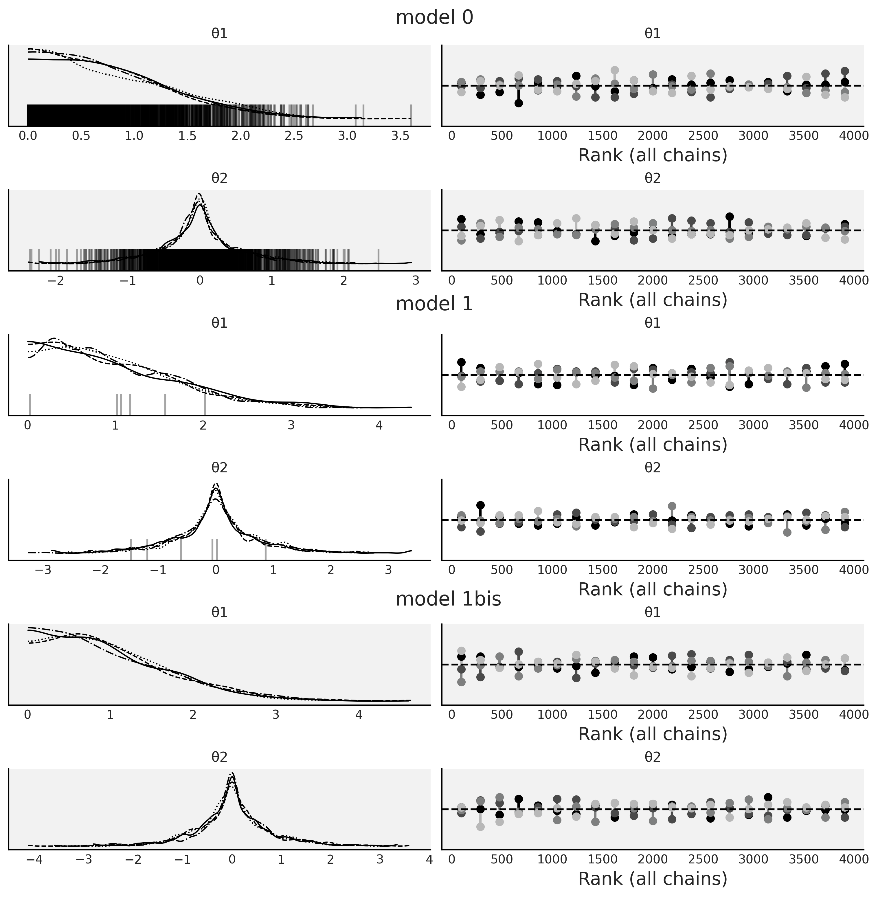
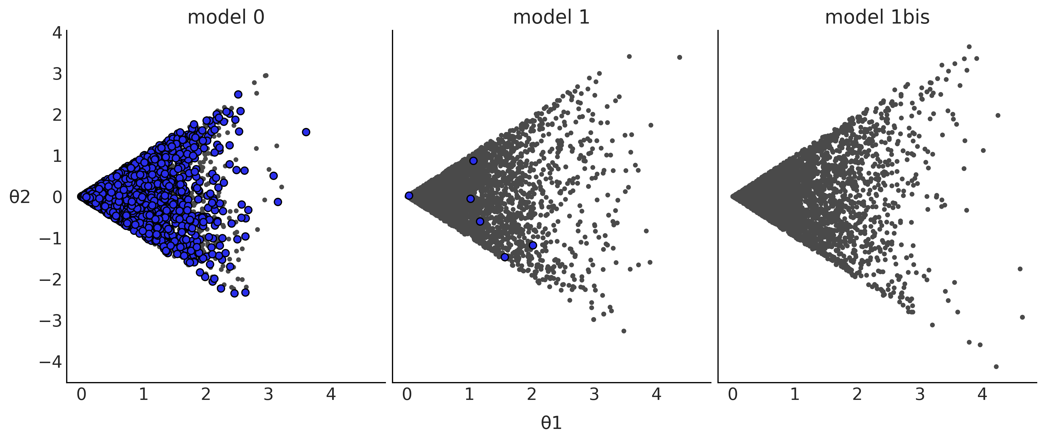
Figure 2.15

_, axes = plt.subplots(1, 3, figsize=(12, 5), sharex=True, sharey=True)

for idata, ax, model in zip(idatas, axes, ["model 0", "model 1", "model 1bis"]):
    az.plot_pair(idata, divergences=True, scatter_kwargs={"color":"C1"}, divergences_kwargs={"color":"C4"}, ax=ax)
    ax.set_xlabel("")
    ax.set_ylabel("")
    ax.set_title(model)
axes[0].set_ylabel('θ2', rotation=0, labelpad=15)
axes[1].set_xlabel('θ1', labelpad=10)
plt.savefig("img/chp02/divergences_pair.png")

Model Comparison

Code 2.15

np.random.seed(90210)

y_obs =  np.random.normal(0, 1, size=100)
idatas_cmp = {}

with pm.Model() as mA:
    σ = pm.HalfNormal("σ", 1)
    y = pm.SkewNormal("y", 0, σ, alpha=1, observed=y_obs)
    idataA = pm.sample(return_inferencedata=True)
    idataA.add_groups({"posterior_predictive": {"y":pm.sample_posterior_predictive(idataA)["y"][None,:]}})
    idatas_cmp["mA"] = idataA

with pm.Model() as mB:
    σ = pm.HalfNormal("σ", 1)
    y = pm.Normal("y", 0, σ, observed=y_obs)
    idataB = pm.sample(return_inferencedata=True)
    idataB.add_groups({"posterior_predictive": {"y":pm.sample_posterior_predictive(idataB)["y"][None,:]}})
    idatas_cmp["mB"] = idataB

with pm.Model() as mC:
    μ = pm.Normal("μ", 0, 1)
    σ = pm.HalfNormal("σ", 1)
    y = pm.Normal("y", μ, σ, observed=y_obs)
    idataC = pm.sample(return_inferencedata=True)
    idataC.add_groups({"posterior_predictive": {"y":pm.sample_posterior_predictive(idataC)["y"][None,:]}})
    idatas_cmp["mC"] = idataC

Auto-assigning NUTS sampler...
Initializing NUTS using jitter+adapt_diag...
Multiprocess sampling (4 chains in 4 jobs)
NUTS: [σ]

100.00% [8000/8000 00:01<00:00 Sampling 4 chains, 0 divergences]

Sampling 4 chains for 1_000 tune and 1_000 draw iterations (4_000 + 4_000 draws total) took 2 seconds.

100.00% [4000/4000 00:04<00:00]

Auto-assigning NUTS sampler...
Initializing NUTS using jitter+adapt_diag...
Multiprocess sampling (4 chains in 4 jobs)
NUTS: [σ]

100.00% [8000/8000 00:01<00:00 Sampling 4 chains, 0 divergences]

Sampling 4 chains for 1_000 tune and 1_000 draw iterations (4_000 + 4_000 draws total) took 2 seconds.

100.00% [4000/4000 00:03<00:00]

Auto-assigning NUTS sampler...
Initializing NUTS using jitter+adapt_diag...
Multiprocess sampling (4 chains in 4 jobs)
NUTS: [σ, μ]

100.00% [8000/8000 00:01<00:00 Sampling 4 chains, 0 divergences]

Sampling 4 chains for 1_000 tune and 1_000 draw iterations (4_000 + 4_000 draws total) took 2 seconds.

100.00% [4000/4000 00:03<00:00]

#3# Table 2.1

cmp = az.compare(idatas_cmp)
cmp.round(2)

/u/32/martino5/unix/anaconda3/envs/pymcv3/lib/python3.9/site-packages/arviz/stats/stats.py:145: UserWarning: The default method used to estimate the weights for each model,has changed from BB-pseudo-BMA to stacking
  warnings.warn(

	rank	loo	p_loo	d_loo	weight	se	dse	warning	loo_scale
mB	0	-137.83	0.92	0.00	1.0	7.07	0.00	False	log
mC	1	-138.57	1.99	0.74	0.0	7.03	0.83	False	log
mA	2	-168.02	1.32	30.20	0.0	10.34	6.55	False	log

Figure 2.16

az.plot_compare(cmp, figsize=(9, 3))
plt.savefig("img/chp02/compare_dummy.png")

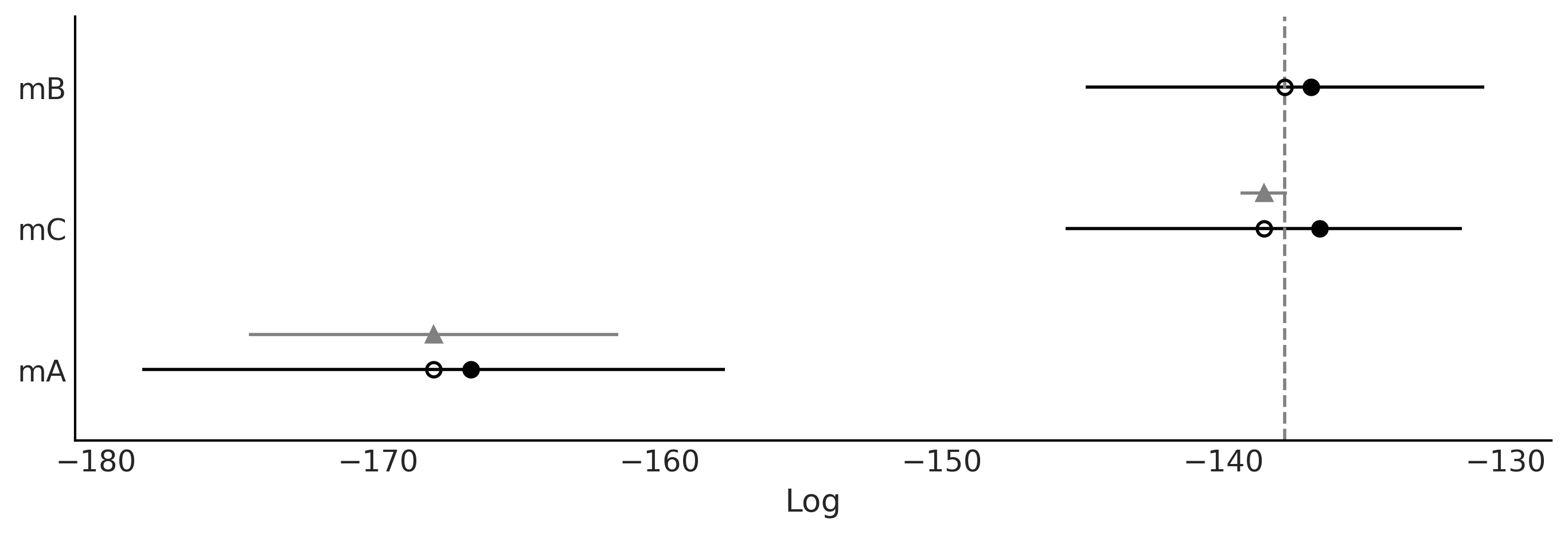
Figure 2.17

az.plot_elpd(idatas_cmp, figsize=(10, 5), plot_kwargs={"marker":"."}, threshold=2);
plt.savefig("img/chp02/elpd_dummy.png")

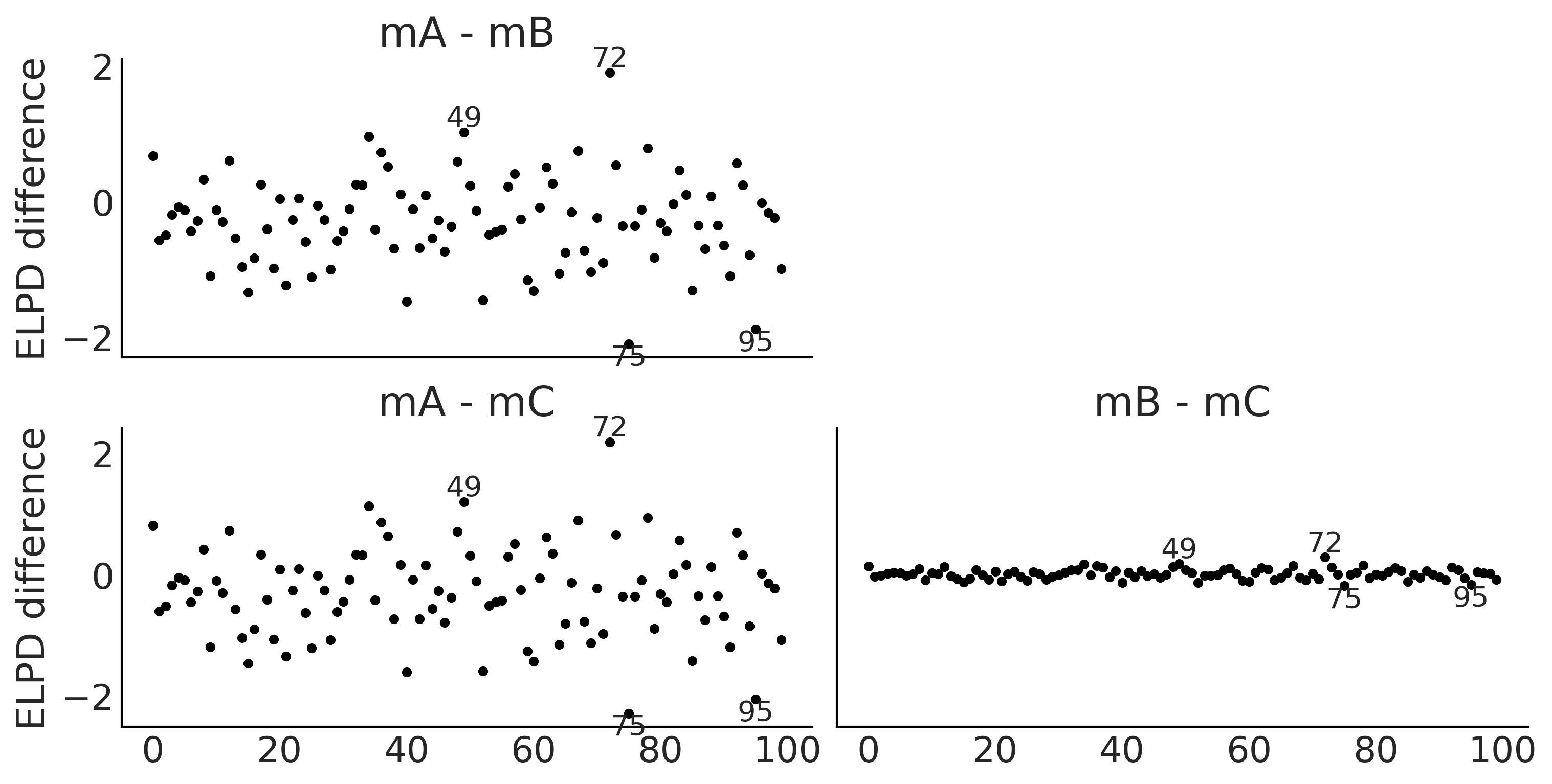
Figure 2.18

_, axes = plt.subplots(1, 3, figsize=(12, 4), sharey=True)
for idx, (model, ax) in enumerate(zip(("mA", "mB", "mC"), axes)):
    loo_ = az.loo(idatas_cmp[model], pointwise=True)
    az.plot_khat(loo_, ax=ax, threshold=0.09, show_hlines=True, hlines_kwargs={"hlines":0.09, "ls":"--"})
    ax.set_title(model)
    if idx:
        axes[idx].set_ylabel("")
    if not idx % 2:
        axes[idx].set_xlabel("")

plt.savefig("img/chp02/loo_k_dummy.png")

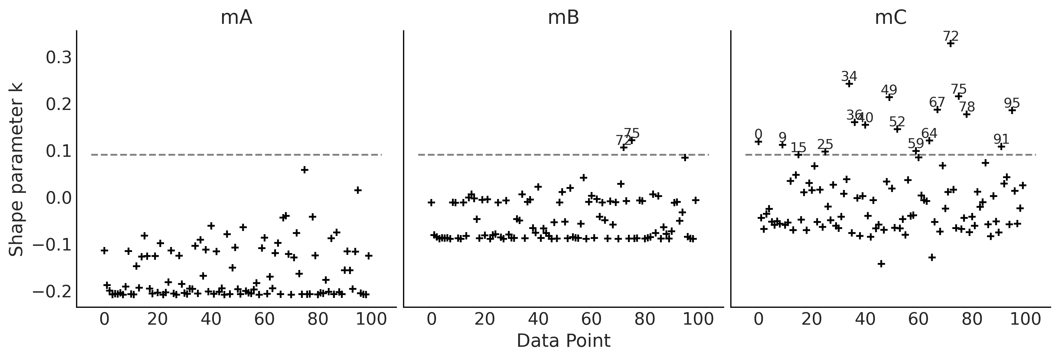
Figure 2.19

az.plot_kde(y_obs, rug=True)
plt.yticks([])
for da, loc in zip([34, 49, 72, 75, 95], [-0.065, -0.05, -0.065, -0.065, -0.065]):
    plt.text(y_obs[da], loc, f"{da}")

plt.text(y_obs[78], loc, "78", fontweight='bold');
plt.savefig("img/chp02/elpd_and_khat.png")

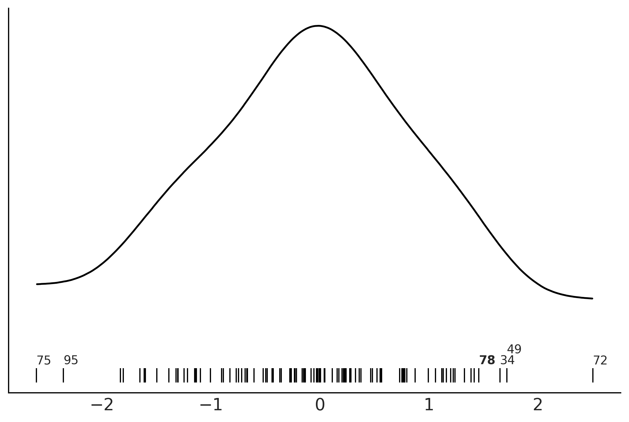
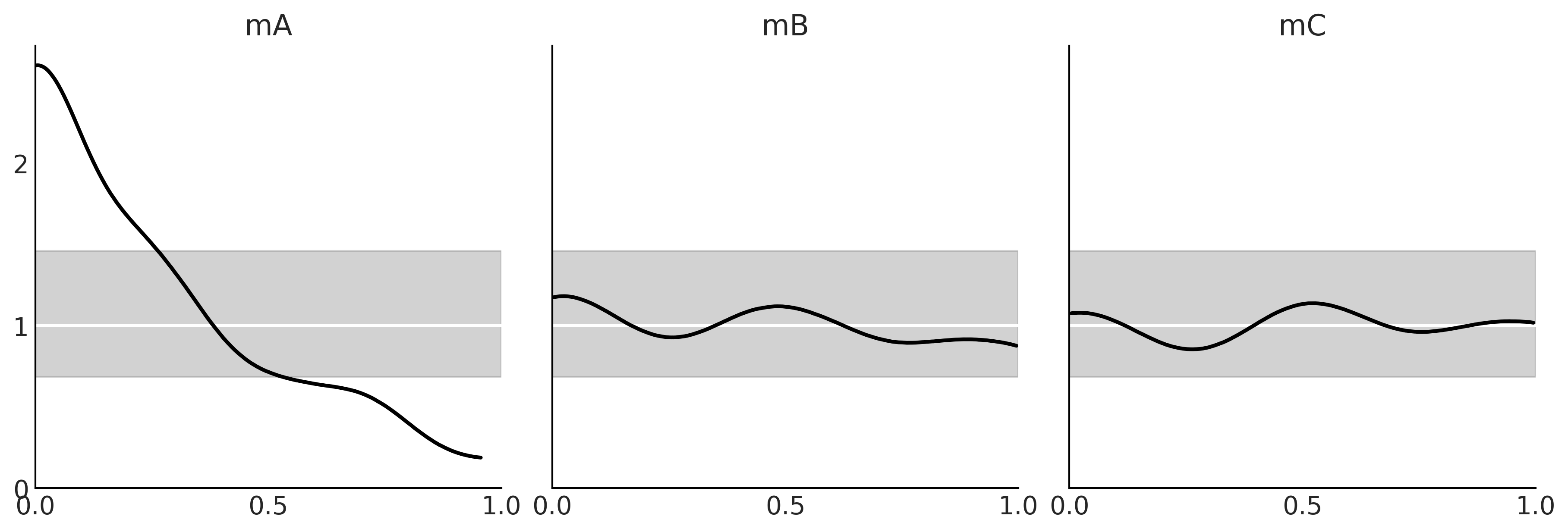
Figure 2.20

_, axes = plt.subplots(1, 3, figsize=(12, 4), sharey=True)
for model, ax in zip(("mA", "mB", "mC"), axes):
    az.plot_loo_pit(idatas_cmp[model], y="y", legend=False, use_hdi=True, ax=ax)
    ax.set_title(model)
    ax.set_xticks([0, 0.5, 1])
    ax.set_yticks([0, 1, 2])

plt.savefig("img/chp02/loo_pit_dummy.png")