11. Appendiceal Topics#
This chapter is different from the rest because it is not about any specific topic. Instead it is a collection of different topics that provide support for the rest of the book by complementing topics discussed in other chapters. These topics are here for readers who are interested in going deeper into each of the methods and theory. In terms of writing style it will be a little bit more theoretical and abstract than other chapters.
11.1. Probability Background#
The Spanish word azahar (the flower of certain critics) and azar (randomness) are not similar out of pure luck. They both come from the Arabic language [1]. From ancient times, and even today, certain games of chance use a bone that it has two flat sides. This bone is similar to a coin or a two-side die. To make it easier to identify one side from the other, at least one side has a distinctive mark, for example, ancient Arabs commonly used a flower. With the passage of time Spanish adopted the term azahar for certain flowers and azar to mean randomness. One of the motivation to the development of probability theory can be track back to understanding games of chance and probably trying to make an small fortune in the process. So let us start this brief introduction to some of the central concepts in probability theory[2] imagining a 6-sided die. Each time we roll the die it is only possible to obtain an integer from 1 to 6 without preference of one over another. Using Python we can program a die like this in the following way:
def die():
    outcomes = [1, 2, 3, 4, 5, 6]
    return np.random.choice(outcomes)
Suppose we suspect that the die is biased. What could we do to evaluate this possibility? A scientific way to answer this question is to collect data and analyze it. Using Python we can simulate the data collection as in Code Block experiment.
def experiment(N=10):
    sample = [die() for i in range(N)]

    for i in range(1, 7):
        print(f"{i}: {sample.count(i)/N:.2g}")

experiment()
1: 0
2: 0.1
3: 0.4
4: 0.1
5: 0.4
6: 0
The numbers in the first column are the possible outcomes. Those in the
second column correspond to the frequency with which each number
appears. Frequency is the number of times each of the possible outcomes
appears divided by N, the total number of times we roll the die.
There are at least two things to take note of in this example. First if
we execute experiment() several times, we will see that we obtain a
different result each time. This is precisely the reason for using dice
in games of chance, every time we roll them we get a number that we
cannot predict. Second, if we roll the same die many times, the ability
to predict each single outcome does not improve. Nevertheless, data
collection and analysis can actually help us to estimate the list of
frequencies for the outcomes, in fact the ability improves as the value
of N increases. Run the experiment for N=10000 times you will see
that the frequencies obtained are approximately \(0.17\) and it turns out
that \(0.17 \approx \frac{1}{6}\) which is what we would expect if each
number on the die had the same chance.
These two observations are not restricted to dice and games of chance. If we weigh ourselves every day we would obtain different values, since our weight is related to the amount of food we eat, the water we drink, how many times we went to the bathroom, the precision of the scale, the clothes we wear and many other factors. Therefore, a single measurement may not be representative of our weight. Of course it could be that the variations are small and we do not consider them important, but we are getting ahead of ourselves. At this point what matters is that the data measurement and/or collection is accompanied by uncertainty. Statistics is basically the field concerned with how to deal with uncertainty in practical problems and Probability theory is one of the theoretical pillars of statistics. Probability theory help us formalize discussion like the one we just had and extend them beyond dice. This is so we can better ask and answer questions related to expected outcomes, such as what happens when we increase the number of experiments, what event has higher chance than another, etc.
11.1.1. Probability#
Probability is the mathematical device that allow us to quantify uncertainty in a principled way. Like other mathematical objects and theories, they can be justified entirely from a pure mathematical perspective. Nevertheless, from a practical point of view we can justify them as naturally arising from performing experiments, collecting observational data and even when doing computational simulations. For simplicity we will talk about experiments, knowing we are using this term in a very broad sense. To think about probabilities we can think in terms of mathematical sets. The sample space \(\mathcal{X}\) is the set of all possible events from an experiment. An event \(A\) is a subset of \(\mathcal{X}\). We say \(A\) happens when we perform an experiment and we get \(A\) as the outcome. For a typical 6 face die we can write:
We may define the event \(A\) as any subset of \(\mathcal{X}\), for example, getting an even number, \(A = \{2, 4, 6\}\). We can associate probabilities to events. If we want to indicate the probability of the event \(A\) we write \(P(A=\{2, 4, 6\})\) or to be more concise \(P(A)\). The probability function \(P\) takes an event \(A\) which is a subset of \(\mathcal{X}\) as input and returns \(P(A)\). Probabilities, like \(P(A)\), can take any number in the interval 0 to 1 (including both extremes), using interval notation we write this is as \([0, 1]\), the brackets meaning inclusive bounds. If the event never happens then the probability of that event is 0, for example \(P(A=-1)=0\), if the event always happens then it has probability 1, for example \(P(A=\{1,2,3,4,5,6\})=1\). We say events are disjoint if they can not happen together, for example, if the event \(A_1\) represent odds numbers and \(A_2\) even numbers, then the probability of rolling a die an getting both \(A_1\) and \(A_2\) is 0. If the event \(A_1, A_2, \cdots A_n\) are disjoint, meaning they can not happen at the same time, then \(\sum_i^n P(A_i) = 1\). Continuing with the example of \(A_1\) representing odd numbers and \(A_2\) even numbers, then the probability of rolling a die and getting either \(A_1\) or \(A_2\) is 1. Any function that satisfies these properties is a valid probability function. We can think of probability as a positive, conserved quantity that is allocated across the possible events [3].
As we just saw, probabilities have a clear mathematical definition. How we interpret probabilities is a different story with different schools of thought. As Bayesian we tend to interpret probabilities as degrees of uncertainty. For example, for a fair die, the probability of getting an odd number when rolling a die is \(0.5\), meaning we are half-sure we will get an odd number. Alternatively we can interpret this number as saying if we roll a die infinite times, half the time we will get odd numbers and half the time even numbers. This is the frequentist interpretation which is also a useful way of thinking about probabilities. If you do not want to roll the die infinite times you can just roll it a large number of times and say that you will approximately get odds half of the time. This is in fact what we did in Code Block experiment. Finally, we notice that for a fair die we expect the probability of getting any single number to be \(\frac{1}{6}\), but for a non-fair die this probability may be different. The equiprobability of the outcomes is just a special case.
If probabilities reflect uncertainty, then is natural to ask what is the probability that the mass of Mars is \(6.39 \times 10^{23}\) kg, or the probability of rain on May 1 in Helsinki, or the probability that capitalism gets replaced by a different socio-economical system in the next 3 decades. We say this definition of probability is epistemic, since it is not about a property of the real world (whatever that is) but a property about our knowledge about that world. We collect data and analyze it, because we think that we can update our internal knowledge state based on external information.
We notice that what can happen in the real world is determined by all the details of the experiments, even those we do not control or are not aware of. On the contrary the sample space is a mathematical object that we define either implicitly or explicitly. For example, by defining the sample space of our die as in Equation (11.1) we are ruling out the possibility of the die landing on an edge, which is actually possible when rolling dice in a non-flat surface. Elements from the sample space may be excluded on purpose, for example, we may have designed the experiment in such a way that we roll the die until we get one integer from \(\{1, 2, 3, 4, 5, 6\}\). Or by omission, like in a survey we may ask people about their gender, but if we only include female or male as options in the possible response, we may force people to choose between two non-adequate answers or completely miss their answers as they may not feel interested in responding to the rest of the survey. We must be aware that the platonic world of ideas which includes all mathematical concepts is different from the real world, in statistical modeling we constantly switch back and forth between these two worlds.
11.1.2. Conditional Probability#
Given two events \(A\) and \(B\) with \(P(B) > 0\), the probability of \(A\) given \(B\), which we write as \(P(A \mid B)\) is defined as :
\(P(A, B)\) is the probability that the events \(A\) and \(B\) occur, it is also usually written as \(P(A \cap B)\) (the symbol \(\cap\) indicates intersection of sets), the probability of the intersection of the events \(A\) and \(B\).
\(P(A \mid B)\) it is known as conditional probability, and it is the probability that event \(A\) occurs, conditioned by the fact that we know (or assume, imagine, hypothesize, etc) that \(B\) has occurred. For example, the probability that a sidewalk is wet is different from the probability that such a sidewalk is wet given that it is raining.
A conditional probability can be viewed as the reduction or restriction of the sample space. Fig. 11.1 shows how we went from having the events \(A\) and \(B\) in the sample space \(\mathcal{X}\), on the left, to having \(B\) as the sample space and a subset of \(A\), the one being compatible with \(B\). When we say that \(B\) has occurred we are not necessarily talking about something in the past, it is just a more colloquial way of saying, once we have conditioned on \(B\) or once we have restricted the sample space to agree with the evidence \(B\).
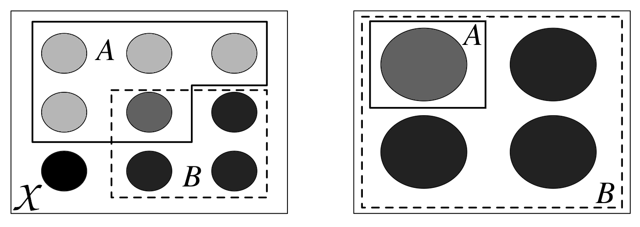
Fig. 11.1 Conditioning is redefining the sample space. On the left we see the sample \(\mathcal{X}\), each circle represent a possible outcome. We have two events, \(A\) and \(B\). On the right we have represented \(P(A \mid B)\), once we know \(B\) we can rule out all events not in \(B\). This figure was adapted from Introduction to Probability [5].#
The concept of conditional probability is at the heart of statistics and is central to thinking about how we should update our knowledge of an event in the light of new data. All probabilities are conditional, with respect to some assumption or model. Even when we do not express it explicitly, there are no probabilities without context.
11.1.3. Probability Distribution#
Instead of calculating the probability of obtaining the number 5 when rolling a die, we may be more interested in finding out the list of probabilities for all numbers on a die. Once this list is computed we can display it or use it to compute other quantities like the probability of getting the number 5, or the probability of getting a number equal or larger than 5. The formal name of this list is probability distribution.
Using Code Block experiment we obtained an empirical probability distribution of a die, that is, a distribution calculated from data. But there are also theoretical distributions, which are central in statistics among other reasons because they allow the construction of probabilistic models.
Theoretical probability distributions have precise mathematical formulas, similar to how circles have a precise mathematical definition. A circle is the geometric space of points on a plane that are equidistant from another point called the center. Given the parameter radius, a circle is perfectly defined [4]. We could say that there is not a single circumference, but a family of circumferences where each member differs from the rest only by the value of the parameter radius, since once this parameter is also defined, the circumference is defined.
Similarly, probability distributions come in families, whose members are perfectly defined by one or more parameters. It is common to write the parameter names with letters of the Greek alphabet, although this is not always the case. Fig. 11.2 is an example of such families of distributions, that we may use to represent a loaded die. We can see how this probability distribution is controlled by two parameters \(\alpha\) and \(\beta\). If we change them the shape of the distribution changes, we can make it flat or concentrated towards one side, push most of the mass the extremes, or concentrated the mass in the middle. As the radius of the circumference is restricted to be positive, the parameters of distributions also have restrictions, in fact \(\alpha\) and \(\beta\) must both be positive.
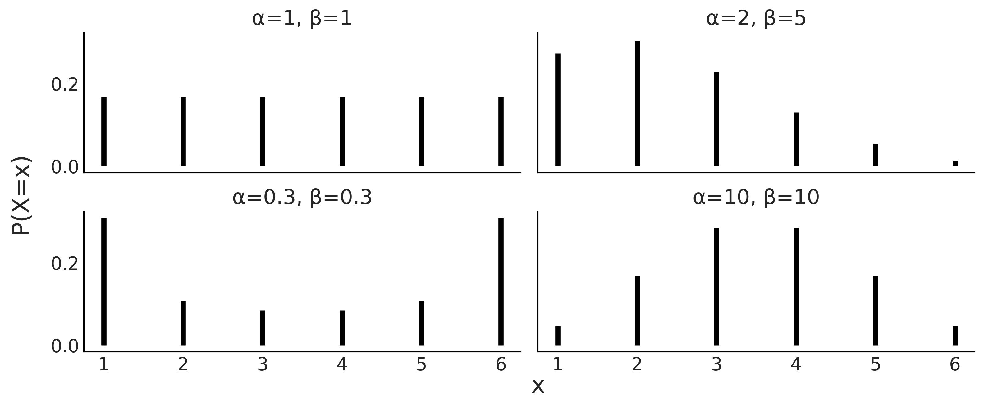
Fig. 11.2 Four members of a family of discrete distributions with parameters \(\alpha\) and \(\beta\). The height of the bars represents the probability of each \(x\) value. The values of \(x\) not drawn have probability 0 as they are out of the support of the distribution.#
11.1.4. Discrete Random Variables and Distributions#
A random variable is a function that maps the sample space into the real numbers \(\mathbb{R}\). Continuing with the die example if the events of interest were the number of the die, the mapping is very simple, we associate \(\LARGE \unicode{x2680}\) with the number 1, \(\LARGE \unicode{x2681}\) with 2, etc. With two dice we could have an \(S\) random variable as the sum of the outcomes of both dice. Thus the domain of the random variable \(S\) is \(\{2, 3, 4, 5, 6, 7, 8, 9, 10, 11, 12\}\), and if both dice are fair then their probability distribution is depicted in Fig. 11.3.
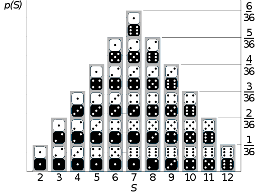
Fig. 11.3 If the sample space is the set of possible numbers rolled on two dice, and the random variable of interest is the sum \(S\) of the numbers on the two dice, then \(S\) is a discrete random variable whose distribution is described in this figure with the probability of each outcome represented as the height of the columns. This figure has been adapted from https://commons.wikimedia.org/wiki/File:Dice_Distribution_(bar).svg#
.svg)
We could also define another random variable \(C\) with sample space \(\{\text{red}, \text{green}, \text{blue}\}\). We could map the sample space to \(\mathbb{R}\) in the following way:
This encoding is useful, because performing math with numbers is easier than with strings regardless of whether we are using analog computation on “pen and paper” or digital computation with a computer.
As we said a random variable is a function, and given that the mapping between the sample space and \(\mathbb{R}\) is deterministic it is not immediately clear where the randomness in a random variable comes from. We say a variable is random in the sense that if we perform an experiment, i.e. we ask the variable for a value like we did in Code Block die and experiment we will get a different number each time without the succession of outcomes following a deterministic pattern. For example, if we ask for the value of random variable \(C\) 3 times in a row we may get red, red, blue or maybe blue, green, blue, etc.
A random variable \(X\) is said to be discrete if there is a finite list of values \(a_1, a_2, \dots, a_n\) or an infinite list of values \(a_1, a_2, \dots\) such that the total probability is \(\sum_j P(X=a_j) = 1\). If \(X\) is a discrete random variable then a finite or countably infinite set of values \(x\) such that \(P(X = x) > 0\) is called the support of \(X\).
As we said before we can think of a probability distribution as a list associating a probability with each event. Additionally a random variable has a probability distribution associated to it. In the particular case of discrete random variables the probability distribution is also called a Probability Mass Function (PMF). It is important to note that the PMF is a function that returns probabilities. The PMF of \(X\) is the function \(P(X=x)\) for \(x \in \mathbb{R}\). For a PMF to be valid, it must be non-negative and sum to 1, i.e. all its values should be non-negative and the sum over all its domain should be 1.
It is important to remark that the term random in random variable does not implies that any value is allowed, only those in the sample space. For example, we can not get the value orange from \(C\), nor the value 13 from \(S\). Another common source of confusion is that the term random implies equal probability, but that is not true, the probability of each event is given by the PMF, for example, we may have \(P(C=\text{red}) = \frac{1}{2}, P(C=\text{green}) = \frac{1}{4}, P(C=\text{blue}) = \frac{1}{4}\). The equiprobability is just a special case.
We can also define a discrete random variable using a cumulative distribution function (CDF). The CDF of a random variable \(X\) is the function \(F_X\) given by \(F_X(x) = P(X \le x)\). For a CDF to be valid, it must be monotonically increasing [5], right-continuous [6], converge to 0 as \(x\) approaches to \(- \infty\), and converge to 1 as \(x\) approaches \(\infty\).
In principle, nothing prevents us from defining our own probability distribution. But there are many already defined distributions that are so commonly used, they have their own names. It is a good idea to become familiar with them as they appear quite often. If you check the models defined in this book you will see that most of them use combinations of predefined probability distributions and only a few examples used custom defined distribution. For example, in Section Approximating Moving Averages Code Block MA2_abc we used a Uniform distribution and two potentials to define a 2D triangular distribution.
Figures Fig. 11.4, Fig. 11.5, and Fig. 11.6, are example of some common discrete distribution represented with their PMF and CDF. On the left we have the PMFs, the height of the bars represents the probability of each \(x\). On the right we have the CDF, here the jump between two horizontal lines at a value of \(x\) represents the probability of \(x\). The figure also includes the values of the mean and standard deviation of the distributions, is important to remark that these values are properties of the distributions, like the length of a circumference, and not something that we compute from a finite sample (see Section Expectations for details).
Another way to describe random variables is to use stories. A story for \(X\) describes an experiment that could give rise to a random variable with the same distribution as \(X\). Stories are not formal devices, but they are useful anyway. Stories have helped humans to make sense of their surrounding for millennia and they continue to be useful today, even in statistics. In the book Introduction to Probability [5] Joseph K. Blitzstein and Jessica Hwang make extensive use of this device. They even use story proofs extensively, these are similar to mathematical proof but they can be more intuitive. Stories are also very useful devices to create statistical models, you can think about how the data may have been generated, and then try to write that down in statistical notation and/or code. We do this, for example, in Chapter 9 with our flight delay example.
11.1.4.1. Discrete Uniform Distribution#
This distribution assigns equal probability to a finite set of consecutive integers from interval a to b inclusive. Its PMF is:
for values of \(x\) in the interval \([a, b]\), otherwise \(P(X = x) = 0\), where \(n=b-a+1\) is the total number values that \(x\) can take.
We can use this distribution to model, for example, a fair die. Code Block scipy_unif shows how we can use Scipy to define a distribution and then compute useful quantities such as the PMF, CDF, and moments (see Section Expectations).
a = 1
b = 6
rv = stats.randint(a, b+1)
x = np.arange(1, b+1)

x_pmf = rv.pmf(x)  # evaluate the pmf at the x values
x_cdf = rv.cdf(x)  # evaluate the cdf at the x values
mean, variance = rv.stats(moments="mv")
Using Code Block scipy_unif plus a few lines of Matplotlib we generate Fig. 11.4. On the left panel we have the PMF where the height of each point indicates the probability of each event, we use points and dotted lines to highlight that the distribution is discrete. On the right we have the CDF, the height of the jump at each value of \(x\) indicates the probability of that value.
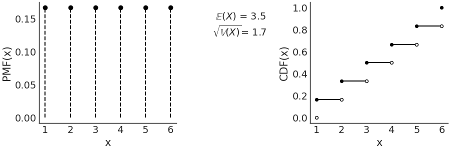
Fig. 11.4 Discrete Uniform with parameters (1, 6). On the left the PMF. The height of the lines represents the probabilities for each value of \(x\). On the right the CDF. The height of the jump at each value of \(x\) represent its probability. Values outside of the support of the distribution are not represented. The filled dots represent the inclusion of the CDF value at a particular \(x\) value, the open dots reflect the exclusion.#
In this specific example the discrete Uniform distribution is defined on the interval \([1, 6]\). Therefore, all values less than 1 and greater than 6 have probability 0. Being a Uniform distribution, all the points have the same height and that height is \(\frac{1}{6}\). There are two parameters of the Uniform discrete distribution, the lower limit \(a\) and upper limit \(b\).
As we already mentioned in this chapter if we change the parameters of a
distribution the particular shape of the distribution will change (try
for example, replacing stats.randint(1, 7) in Code Block
scipy_unif with stats.randint(1, 4). That
is why we usually talk about family of distributions, each member of
that family is a distribution with a particular and valid combination of
parameters. Equation (11.3) defines the family of discrete
Uniform distributions as long as \(a < b\) and both \(a\) and \(b\) are
integers.
When using probability distributions to create statistical applied models it is common to link the parameters with quantities that make physical sense. For example, in a 6 sided die it makes sense that \(a=1\) and \(b=6\). In probability we generally know the values of these parameters while in statistics we generally do not know these values and we use data to infer them.
11.1.4.2. Binomial Distribution#
A Bernoulli trial is an experiment with only two possible outcomes yes/no (success/failure, happy/sad, ill/healthy, etc). Suppose we perform \(n\) independent [7] Bernoulli trials, each with the same success probability \(p\) and let us call \(X\) the number of success. Then the distribution of \(X\) is called the Binomial distribution with parameters \(n\) and \(p\), where \(n\) is a positive integer and \(p \in [0, 1]\). Using statistical notation we can write \(X \sim Bin(n, p)\) to mean that \(X\) has the Binomial distribution with parameters \(n\) and \(p\), with the PMF being:
The term \(p^x(1-p)^{n-x}\) counts the number of \(x\) success in \(n\) trials. This term only considers the total number of success but not the precise sequence, for example, \((0,1)\) is the same as \((1,0)\), as both have one success in two trials. The first term is known as Binomial Coefficient and computes all the possible combinations of \(x\) elements taken from a set of \(n\) elements.
The Binomial PMFs are often written omitting the values that return 0, that is the values outside of the support. Nevertheless it is important to be sure what the support of a random variable is in order to avoid mistakes. A good practice is to check that PMFs are valid, and this is essential if we are proposing a new PMFs instead of using one off the shelf.
When \(n=1\) the Binomial distribution is also known as the Bernoulli distribution. Many distributions are special cases of other distributions or can be obtained somehow from other distributions.
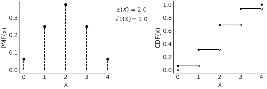
Fig. 11.5 \(\text{Bin}(n=4, p=0.5)\) On the left the PMF. The height of the lines represents the probabilities for each value of \(x\). On the right the CDF. The height of the jump at each value of \(x\) represent its probability. Values outside of the support of the distribution are not represented.#
11.1.4.3. Poisson Distribution#
This distribution expresses the probability that \(x\) events happen during a fixed time interval (or space interval) if these events occur with an average rate \(\mu\) and independently from each other. It is generally used when there are a large number of trials, each with a small probability of success. For example
Radioactive decay, the number of atoms in a given material is huge, the actual number that undergo nuclear fission is low compared to the total number of atoms.
The daily number of car accidents in a city. Even when we may consider this number to be high relative to what we would prefer, it is low in the sense that every maneuver that the driver performs, including turns, stopping at lights, and parking, is an independent trial where an accident could occur.
The PMF of a Poisson is defined as:
Notice that the support of this PMF are all the natural numbers, which is an infinite set. So we have to be careful with our list of probabilities analogy, as summing an infinite series can be tricky. In fact Equation (11.5) is a valid PMF because of the Taylor series \(\sum_0^{\infty} \frac{\mu^{x}}{x!} = e^{\mu}\)
Both the mean and variance of the Poisson distribution are defined by \(\mu\). As \(\mu\) increases, the Poisson distribution approximates to a Normal distribution, although the latter is continuous and the Poisson is discrete. The Poisson distribution is also closely related to the Binomial distribution. A Binomial distribution can be approximated with a Poisson, when \(n >> p\) [8], that is, when the probability of success (\(p\)) is low compared with the number o trials (\(n\)) then \(\text{Pois}(\mu=np) \approx \text{Bin}(n, p)\). For this reason the Poisson distribution is also known as the law of small numbers or the law of rare events. As we previously mentioned this does not mean that \(\mu\) has to be small, but instead that \(p\) is low with respect to \(n\).
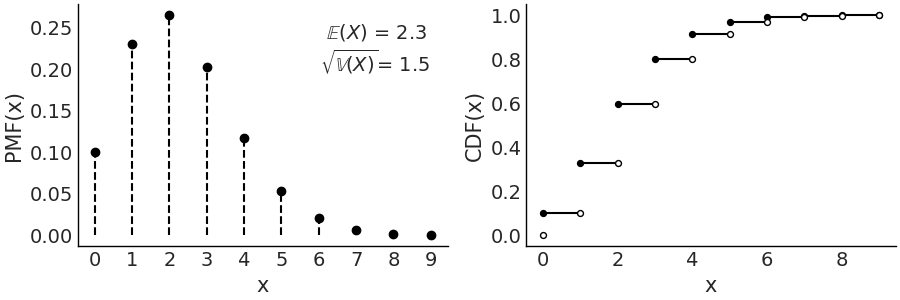
Fig. 11.6 \(\text{Pois}(2.3)\) On the left the PMF. The height of the lines represents the probabilities for each value of \(x\). On the right the CDF. The height of the jump at each value of \(x\) represent its probability. Values outside of the support of the distribution are not represented.#
11.1.5. Continuous Random Variables and Distributions#
So far we have seen discrete random variables. There is another type of random variable that is widely used called continuous random variables, whose support takes values in \(\mathbb {R}\). The most important difference between discrete and continuous random variables is that the latter can take on any \(x\) value in an interval, although the probability of any \(x\) value is exactly 0. Introduced this way you may think that these are the most useless probability distributions ever. But that is not the case, the actual problem is that our analogy of treating a probability distribution as a finite list is a very limited analogy and it fails badly with continuous random variables [9].
In Figures Fig. 11.4, Fig. 11.5, and Fig. 11.6, to represent PMFs (discrete variables), we used the height of the lines to represent the probability of each event. If we add the heights we always get 1, that is, the total sum of the probabilities. In a continuous distribution we do not have lines but rather we have a continuous curve, the height of that curve is not a probability but a probability density and instead of of a PMF we use a Probability Density Function (PDF). One important difference is that height of \(\text{PDF}(x)\) can be larger than 1, as is not the probability value but a probability density. To obtain a probability from a PDF instead we must integrate over some interval:
Thus, we can say that the area below the curve of the PDF (and not the height as in the PMF) gives us a probability, the total area under the curve, i.e. evaluated over the entire support of the PDF, must integrate to 1. Notice that if we want to find out how much more likely the value \(x_1\) is compared to \(x_2\) we can just compute \(\frac{pdf(x_1)}{pdf(x_2)}\).
In many texts, including this one, it is common to use the symbol \(p\) to talk about the \(pmf\) or \(pdf\). This is done in favour of generality and hoping to avoid being very rigorous with the notation which can be an actual burden when the difference can be more or less clear from the context.
For a discrete random variable, the CDF jumps at every point in the support, and is flat everywhere else. Working with the CDF of a discrete random variable is awkward because of this jumpiness. Its derivative is almost useless since it is undefined at the jumps and 0 everywhere else. This is a problem for gradient-based sampling methods like Hamiltonian Monte Carlo (Section Inference Methods). On the contrary for continuous random variables, the CDF is often very convenient to work with, and its derivative is precisely the probability density function (PDF) that we have discussed before.
Fig. 11.7 summarize the relationship between the CDF,
PDF and PMF. The transformations between discrete CDF and PMF on one
side and continuous CDF and PMF on the other are well defined and thus
we used arrows with solid lines. Instead the transformations between
discrete and continuous variables are more about numerical approximation
than well defined mathematical operations. To approximately get from a
discrete to a continuous distribution we use a smoothing method. One
form of smoothing is to use a continuous distribution instead of a
discrete one. To go from continuous to discrete we can discretize or bin
the continuous outcomes. For example, a Poisson distribution with a
large value of \(\mu\) approximately Gaussian [10], while still being
discrete. For those cases using a scenarios using a Poisson or a
Gaussian maybe be interchangeable from a practical point of view. Using
ArviZ you can use az.plot_kde with discrete data to approximate a
continuous functions, how nice the results of this operation look
depends on many factors. As we already said it may look good for a
Poisson distribution with a relatively large value of \(\mu\). When
calling az.plot_bpv(.) for a discrete variable, ArviZ will smooth it,
using an interpolation method, because the probability integral
transform only works for continuous variables.
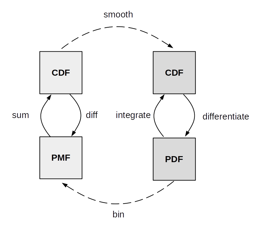
Fig. 11.7 Relationship between the CDF, PDF and PMF. Adapted from the book Think Stats [132].#
As we did with the discrete random variables, now we will see a few example of continuous random variables with their PDF and CDF.
11.1.5.1. Continuous Uniform Distribution#
A continuous random variable is said to have a Uniform distribution on the interval \((a, b)\) if its PDF is:
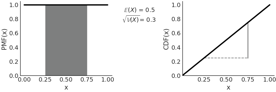
Fig. 11.8 \(\mathcal{U}(0, 1)\) On the left the PDF, the black line represents the probability density, the gray shaded area represents the probability \(P(0.25 < X < 0.75) =0.5\). On the right the CDF, the height of the gray continuous segment represents \(P(0.25 < X < 0.75) =0.5\). Values outside of the support of the distribution are not represented.#
The most commonly used Uniform distribution in statistics is \(\mathcal{U}(0, 1)\) also known as the standard Uniform. The PDF and CDF for the standard Uniform are very simple: \(p(x) = 1\) and \(F_{(x)} = x\) respectively, Fig. 11.8 represents both of them, this figure also indicated how to compute probabilities from the PDF and CDF.
11.1.5.2. Gaussian or Normal Distribution#
This is perhaps the best known distribution [11]. On the one hand, because many phenomena can be described approximately using this distribution (thanks to central limit theorem, see Subsection The Central Limit Theorem below). On the other hand, because it has certain mathematical properties that make it easier to work with it analytically.
The Gaussian distribution is defined by two parameters, the mean \(\mu\) and the standard deviation \(\sigma\) as shown in Equation (11.8). A Gaussian distribution with \(\mu=0\) and \(\sigma=1\) is known as the standard Gaussian distribution.
On the left panel of Fig. 11.9 we have the PDF, and on the right we have the CDF. Both the PDF and CDF are represented for the invertal -4, 4, but notice that the support of the Gaussian distribution is the entire real line.
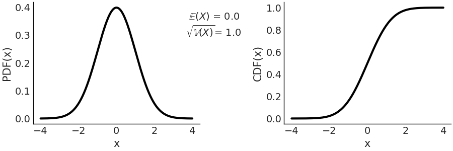
Fig. 11.9 Representation of \(\mathcal{N}(0, 1)\), on the left the PDF, on the right the CDF. The support of the Gaussian distribution is the entire real line.#
11.1.5.3. Student’s t-distribution#
Historically this distribution arose to estimate the mean of a normally distributed population when the sample size is small [12]. In Bayesian statistics, a common use case is to generate models that are robust against aberrant data as we discussed in Section Robust Regression.
where \(\Gamma\) is the gamma function [13] and \(\nu\) is commonly called degrees of freedom. We also like the name degree of normality, since as \(\nu\) increases, the distribution approaches a Gaussian. In the extreme case of \(\lim_{\nu \to \infty}\) the distribution is exactly equal to a Gaussian distribution with the same mean and standard deviation equal to \(\sigma\).
When \(\nu=1\) we get the Cauchy distribution [14]. Which is similar to a Gaussian but with tails decreasing very slowly, so slowly that this distribution does not have a defined mean or variance. That is, it is possible to calculate a mean from a data set, but if the data came from a Cauchy distribution, the spread around the mean will be high and this spread will not decrease as the sample size increases. The reason for this strange behavior is that distributions, like the Cauchy, are dominated by the tail behavior of the distribution, contrary to what happens with, for example, the Gaussian distribution.
For this distribution \(\sigma\) is not the standard deviation, which as already said could be undefined, \(\sigma\) is the scale. As \(\nu\) increases the scale converges to the standard deviation of a Gaussian distribution.
On the left panel of Fig. 11.10 we have the PDF, and on the right we have the CDF. Compare with Fig. 11.9, a standard normal and see how the tails are heavier for the Student T distribution with parameter \(\mathcal{T}(\nu=4, \mu=0, \sigma=1)\)
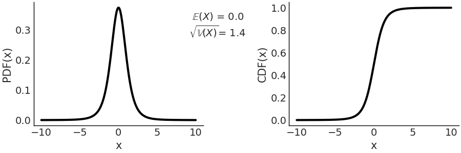
Fig. 11.10 \(\mathcal{T}(\nu=4, \mu=0, \sigma=1)\) On the left the PDF, on the right the CDF. The support of the Students T distribution is the entire real line.#
11.1.5.4. Beta Distribution#
The Beta distribution is defined in the interval \([0, 1]\). It can be used to model the behavior of random variables limited to a finite interval, for example, modeling proportions or percentages.
The first term is a normalization constant that ensures that the PDF integrates to 1. \(\Gamma\) is the Gamma function. When \(\alpha = 1\) and \(\beta = 1\) the Beta distribution reduces to the standard Uniform distribution. In Fig. 11.11 we show a \(\text{Beta}(\alpha=5, \beta=2)\) distribution.
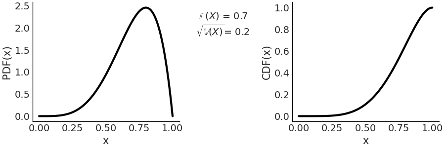
Fig. 11.11 \(\text{Beta}(\alpha=5, \beta=2)\) On the left the PDF, on the right the CDF. The support of the Beta distribution is on the interval \([0, 1]\).#
If we want to express the Beta distribution as a function of the mean and the dispersion around the mean, we can do it in the following way. \(\alpha = \mu \kappa\), \(\beta = (1 - \mu) \kappa\) where \(\mu\) the mean and \(\kappa\) a parameter called concentration as \(\kappa\) increases the dispersion decreases. Also note that \(\kappa = \alpha + \beta\).
11.1.6. Joint, Conditional and Marginal Distributions#
Let us assume we have two random variables \(X\) and \(Y\) with the same PMF \(\text{Bin}(1, 0.5)\). Are they dependent or independent? If \(X\) represent heads in on coin toss and \(Y\) heads in another coin toss then they are independent. But if they represent heads and tails, respectively, on the same coin toss, then they are dependent. Thus even when individual (formally known as univariate) PMFs/PDFs fully characterize individual random variables, they do not have information about how the individual random variables are related to other random variables. To answer that question we need to know the joint distribution, also known as multivariate distributions. If we consider that \(p(X)\) provides all the information about the probability of finding \(X\) on the real line, in a similar way \(p(X, Y)\), the joint distribution of \(X\) and \(Y\), provides all the information about the probability of finding the tuple \((X, Y)\) on the plane. Joint distributions allow us to describe the behavior of multiple random variables that arise from the same experiment, for example, the posterior distribution is the joint distribution of all parameters in the model after we have conditioned the model on observed data.
The joint PMF is given by
The definition for \(n\) discrete random variable is similar, we just need to include \(n\) terms. Similarly to univariate PMFs valid joint PMFs must be nonnegative and sum to 1, where the sum is taken over all possible values.
In a similar way the joint CDF of \(X\) and \(Y\) is
Given the joint distribution of \(X\) and \(Y\), we can get the distribution of \(X\) by summing over all the possible values of \(Y\):
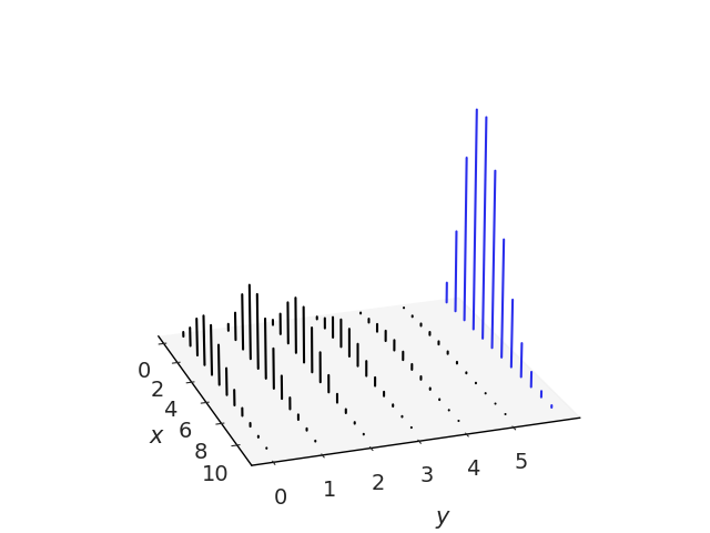
Fig. 11.12 The black lines represent the joint distribution of \(x\) and \(y\). The blue lines in the marginal distribution of \(x\) are obtained by adding the heights of the lines along the y-axis for every value of \(x\).#
In previous section we called \(P(X=x)\) the PMF of \(X\), or just the distribution of \(X\), when working with joint distributions we often call it the marginal distribution of \(X\). We do this to emphasize we are talking about the individual \(X\), without any reference to \(Y\). By summing over all the possible values of \(Y\) we get rid of \(Y\). Formally this process is known as marginalizing out \(Y\). To obtain the PMF of \(Y\) we can proceed in a similar fashion, but summing over all possible values of \(X\) instead. In the case of a joint distribution of more than 2 variables we just need to sum over all the other variables. Fig. 11.12 illustrates this.
Given the joint distribution it is straightforward to get the marginals. But going from the marginals to the joint distribution is not generally possible unless we make further assumptions. In Fig. 11.12 we can see that there is just one way to add heights of the bars along the y-axis or x-axis, but to do the inverse we must split bars and there are infinite ways of making this split.
We already introduced conditional distributions in Section Conditional Probability, and in Fig. 11.1 we show that conditioning is redefining the sample space. Fig. 11.13 demonstrates conditioning in the context of a joint distribution of \(X\) and \(Y\). To condition on \(Y=y\) we take the joint distribution at the \(Y=y\) value and forget about the rest. i.e. those for which \(Y \ne y\), this is similar as indexing a 2d array and picking a single column or row. The remaining values of \(X\), those in bold in Fig. 11.13 needs to sum 1 to be a valid PMF, and thus we re-normalize by dividing by \(P(Y=y)\)
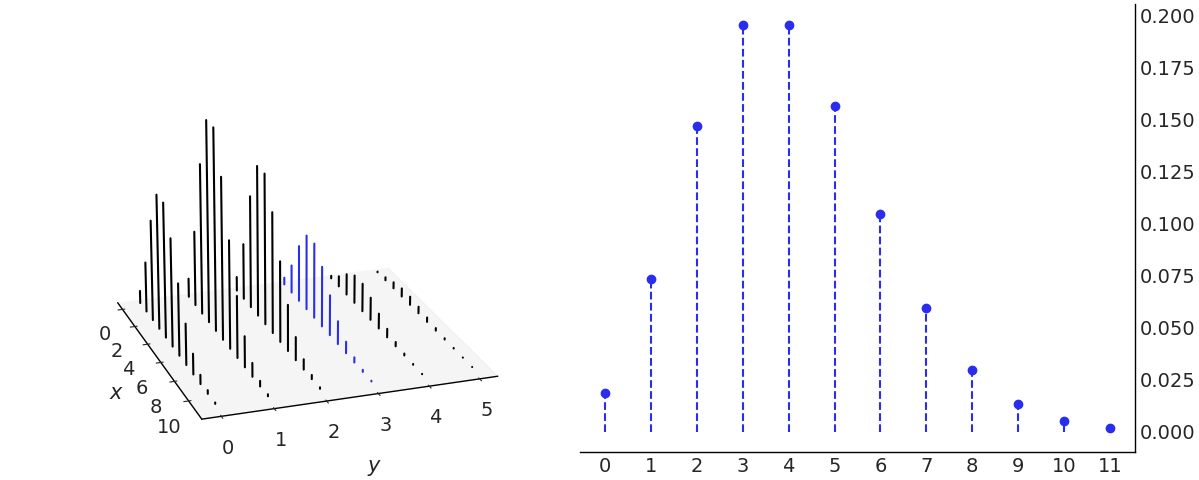
Fig. 11.13 On the left the joint distribution of \(x\) and \(y\). The blue lines represent the conditional distribution \(p(x \ mid y=3)\). On the right we plot the same conditional distribution separately. Notice that there are as many conditional PMF of \(x\) as values of \(y\) and vice versa. We are just highlighting one possibility.#
We define continuous joint CDFs as in Equation (11.13) the same as with discrete variables and the joint PDFs as the derivative of the CDFs with respect to \(x\) and \(y\). We require valid joint PDFs to be nonnegative and integrate to 1. For continuous variables we can marginalize variables out in a similar fashion we did for discrete ones, with the difference that instead of a sum we need to compute an integral.
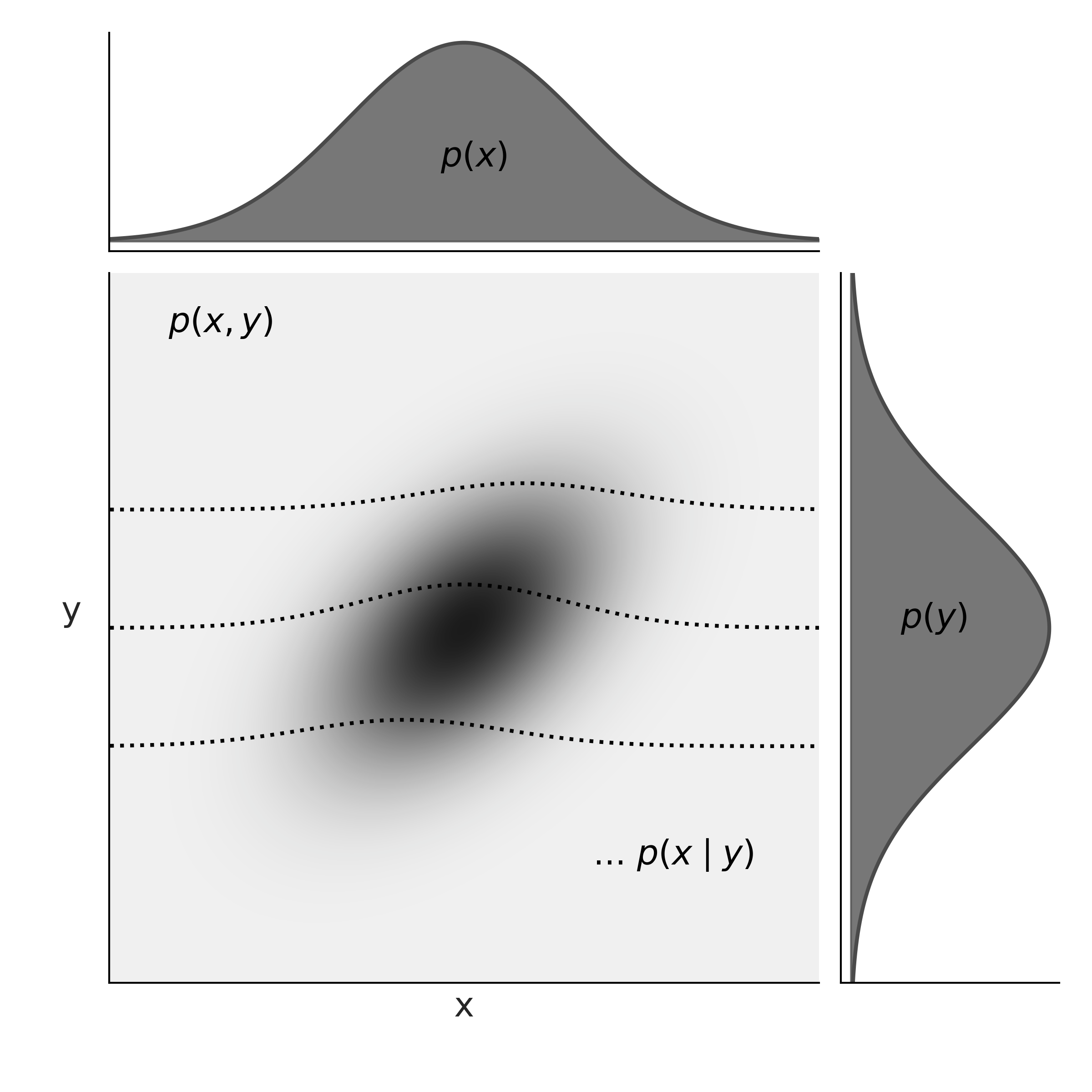
Fig. 11.14 At the center of the figure we have the joint probability \(p(x, y)\) represented with a gray scale, darker for higher probability density. At the top and right margins we have the marginal distributions \(p(x)\) and \(p(y)\) respectively. The dashed lines represents the conditional probability \(p(x \mid y)\) for 3 different values of \(y\). We can think of these as (renormalized) slices of the joint \(p(x, y)\) at a given value of \(y\).#
Fig. 11.15 show another example of a a join distribution with its marginals distribution. This is also a clear example that going from the joint to the marginals is straightforward, as there is a unique way of doing it, but the inverse is not possible unless we introduce further assumptions. Joint distributions can also be a hybrid of discrete and continuous distributions. Fig. 11.16 shows an example.
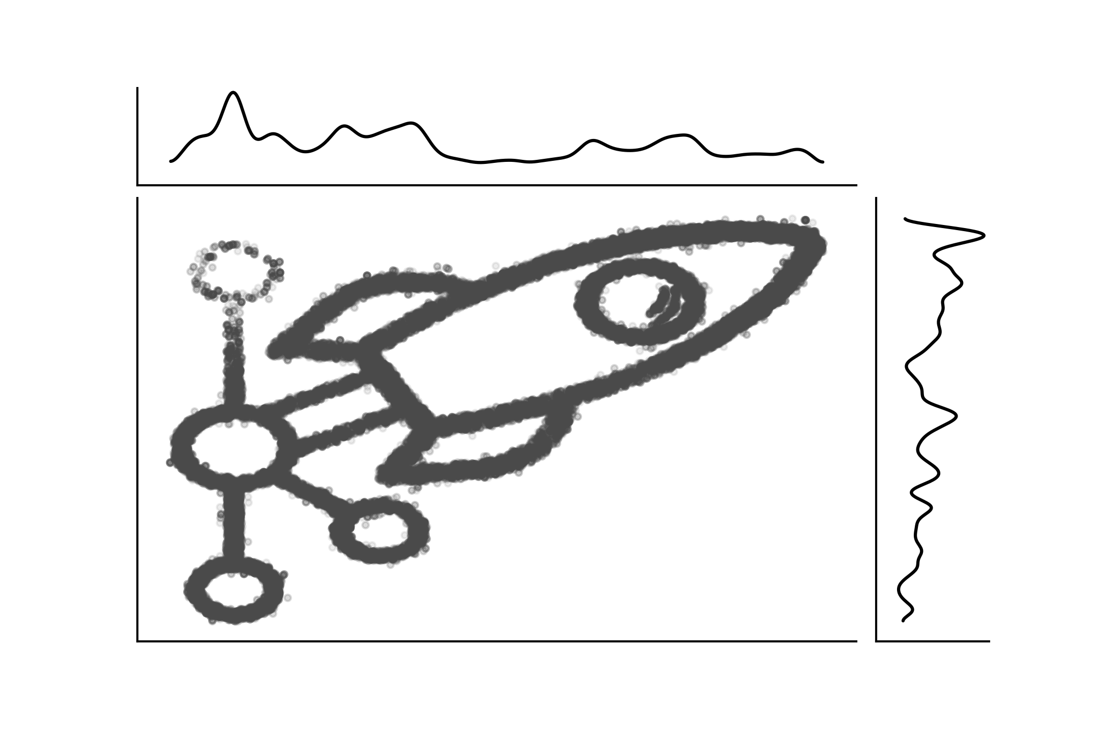
Fig. 11.15 The PyMC3 logo as a sample from a joint distribution with its marginals. This figure was created with imcmc ColCarroll/imcmc a library for turning 2D images into probability distributions and then sampling from them to create images and gifs.#
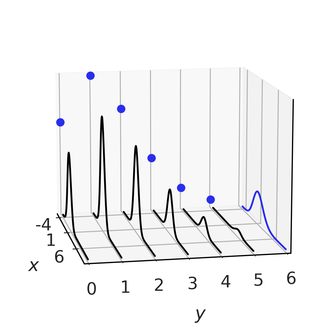
Fig. 11.16 A hybrid joint distribution in black. The marginals are represented in blue, with \(X\) being distributed as a Gaussian and \(Y\) as a Poisson. It is easy to see how for each value of \(Y\) we have a (Gaussian) conditional distribution.#
11.1.7. Probability Integral Transform (PIT)#
The probability integral transform (PIT), also known as the universality of the Uniform distribution, states that given a random variable \(X\) with a continuous distribution with cumulative distribution \(F_X\), we can compute a random variable \(Y\) with standard Uniform distribution as:
We can see this is true as follows, by the definition of the CDF of \(Y\)
Replacing Equation (11.16) in the previous one
Taking the inverse of \(F_X\) to both sides of the inequality
By the definition of CDF
Simplifying, we get the CDF of a standard Uniform distribution \(\mathcal{U}\)(0, 1).
If we do not know the CDF \(F_X\) but we have samples from \(X\) we can approximate it with the empirical CDF. Fig. 11.17 shows example of this property generated with Code Block pit
xs = (np.linspace(0, 20, 200), np.linspace(0, 1, 200), np.linspace(-4, 4, 200))
dists = (stats.expon(scale=5), stats.beta(0.5, 0.5), stats.norm(0, 1))


_, ax = plt.subplots(3, 3)

for idx, (dist, x) in enumerate(zip(dists, xs)):
    draws = dist.rvs(100000)
    data = dist.cdf(draws)
    # PDF original distribution
    ax[idx, 0].plot(x, dist.pdf(x))
    # Empirical CDF
    ax[idx, 1].plot(np.sort(data), np.linspace(0, 1, len(data)))
    # Kernel Density Estimation
    az.plot_kde(data, ax=ax[idx, 2])

Fig. 11.17 On the first column we have the PDF of 3 different distributions. To generate the plots in the middle column, we take 100000 draws from the corresponding PDF compute the CDF for those draws. We can see these are the CDF for the Uniform distribution. The last column is similar to the middle one, except that instead of plotting the empirical CDF we use a a kernel density estimator to approximate the PDF, which we can see that is approximately Uniform. The figure was generated with Code Block pit.#
The probability integral transform is used as part of tests to evaluate
if a given dataset can be modeled as arising from a specified
distribution (or probabilistic model). In this book we have seen PIT
used behind both visual test az.plot_loo_pit() and
az.plot_pbv(kind="u_values").
PIT can also be used to sample from distributions. If the random
variable \(X\) is distributed as \(\mathcal{U}(0,1)\), then \(Y = F^{-1}(X)\)
has the distribution \(F\). Thus to obtain samples from a distribution we
just need (pseudo)random number generator like np.random.rand() and
the inverse CDF of the distribution of interest. This may not be the
most efficient method, but its generality and simplicity are difficult
to beat.
11.1.8. Expectations#
The expectation is a single number summarizing the center of mass of a distribution. For example, if \(X\) is a discrete random variable, then we can compute its expectation as:
As is often the case in statistics we want to also measure the spread, or dispersion, of a distribution, for example, to represent uncertainty around a point estimate like the mean. We can do this with the variance, which itself is also an expectation:
The variance often appears naturally in many computations, but to report results it is often more useful to take the square root of the variance, called the standard deviation, as this will be in the same units as the random variable.
Figures Fig. 11.4, Fig. 11.5, Fig. 11.6, Fig. 11.8, Fig. 11.9, Fig. 11.10, and Fig. 11.11 show the expectation and the standard deviations for different distributions. Notice that these are not values computed from samples but properties of theoretical mathematical objects.
Expectation is linear, meaning that:
where \(c\) is a constant and
which are true even in the case that \(X\) and \(Y\) are dependent. Instead, the variance is not linear:
and in general:
except, for example, when \(X\) and \(Y\) are independent.
We denote the \(n\)th moment of a random variable \(X\) is \(\mathbb{E}(X^n)\), thus the expected value and the variance are also known as the first and second moments of a distribution. The third moment, the skew, tells us about the asymmetry of a distribution. The skewness of a random variable \(X\) with mean \(\mu\) and variance \(\sigma^2\) is the third (standardized moment) of \(X\):
The reason to compute the skew as a standardized quantity, i.e. to subtract the mean and divide by the standard deviation is to make the skew independent of the localization and scale of \(X\), this is reasonable as we already have that information from the mean and variance and also it will make the skewness independent of the units of \(X\), so it becomes easier to compare skewness.
For example, a \(\text{Beta}(2, 2)\) has a 0 skew while for \(\text{Beta}(2, 5)\) the skew is positive and for \(\text{Beta}(5, 2)\) negative. For unimodal distributions, a positive skew generally means that the right tail is longer, and the opposite for a negative skew. This is not always the case, the reason is that a 0 skew means that the total mass at the tails on both sides is balanced. So we can also balance the mass by having one long thin tail an another short and fat tail.
The fourth moment, known as kurtosis, tells us about the behavior of the tails or the extreme values [133]. It is defined as
The reason to subtract 3 is to make the Gaussian have 0 kurtosis, as it is often the case that kurtosis is discussed in comparison with the Gaussian distribution, but sometimes it is often computed without the \(-3\), so when in doubt ask, or read, for the exact definition used in a particular case. By examining the definition of kurtosis in Equation (11.29) we can see that we are essentially computing the expected value of the standardized data raised to the fourth power. Thus any standardized values less than 1 contribute virtually nothing to the kurtosis. Instead the only values that has something to contribute are the extreme values.
As we increase increase the value of \(\nu\) in a Student t distribution the kurtosis decreases (it is zero for a Gaussain distribution) and the kurtosis increases as we decrease \(\nu\). The kurtosis is only defined when \(\nu > 4\), in fact for the Student T distribution the \(n\)th moment is only defined for \(\nu > n\).
The stats module of SciPy offers a method stats(moments) to compute
the moments of distributions as you can see in Code Block
scipy_unif where it is used to obtain the
mean and variance. We notice that all we have discussed in this section
is about computing expectation and moments from probability
distributions and not from samples, thus we are talking about properties
of theoretical distributions. Of course in practice we usually want to
estimate the moments of a distribution from data and for that reason
statisticians have studies estimators, for example, the sample mean and
the sample median are estimators of \(\mathbb{E}(X)\).
11.1.9. Transformations#
If we have a random variable \(X\) and we apply a function \(g\) to it we obtain another random variable \(Y = g(X)\). After doing so we may ask, given that we know the distribution of \(X\) how can we find out the distribution of \(Y\). One easy way of doing it, is by sampling from \(X\) applying the transformation and then plotting the results. But of course there are formals ways of doing it. One such way is applying the change of variables technique.
If \(X\) is a continuous random variable and \(Y = g(X)\), where \(g\) is a differentiable and strictly increasing or decreasing function, the PDF of \(Y\) is:
We can see this is true as follows. Let \(g\) be strictly increasing, then the CDF of \(Y\) is:
and then by the chain rule, the PDF of \(Y\) can be computed from the PDF of \(X\) as:
The proof for \(g\) strictly decreasing is similar but we end up with a minus sign on the right hand term and thus the reason we compute the absolute value in Equation (11.30).
For multivariate random variables (i.e in higher dimensions) instead of the derivative we need to compute the Jacobian determinant, and thus it is common to refer the term \(\left| \frac{dx}{dy} \right|\) as the Jacobian even in the one dimensional case. The absolute value of the Jacobian determinant at a point \(p\) gives us the factor by which a function \(g\) expands or shrinks volumes near \(p\). This interpretation of the Jacobian is also applicable to probability densities. If the transformation \(g\) is not linear then the affected probability distribution will shrink in some regions and expand in others. Thus we need to properly take into account these deformations when computing \(Y\) from the known PDF of \(X\). Slightly rewriting Equation (11.30) like below also helps:
As we can now see that the probability of finding \(Y\) in a tiny interval \(p_Y(y)dy\) is equal to the probability of finding \(X\) in a tiny interval \(p_X(x)dx\). So the Jacobian is telling us how we remap probabilities in the space associated to \(X\) with those associated with \(Y\).
11.1.10. Limits#
The two best known and most widely used theorems in probability are the law of large numbers and the central limit theorem. They both tell us what happens to the sample mean as the sample size increases. They can both be understood in the context of repeated experiments, where the outcome of the experiment could be viewed as a sample from some underlying distribution.
11.1.10.1. The Law of Large Numbers#
The law of large number tells us that the sample mean of an iid random variable converges, as the number of samples increase, to the expected value of the random variable. This is not true for some distributions such as the Cauchy distribution (which has no mean or finite variance).
The law of large numbers is often misunderstood, leading to the gambler’s fallacy. An example of this paradox is believing that it is smart to bet in the lottery on a number that has not appeared for a long time. The erroneous reasoning here is that if a particular number has not appeared for a while then there is must be some kind of force that increases the probability of that number in the next draws. A force that re-establish the equiprobability of the numbers and the natural order of the universe.
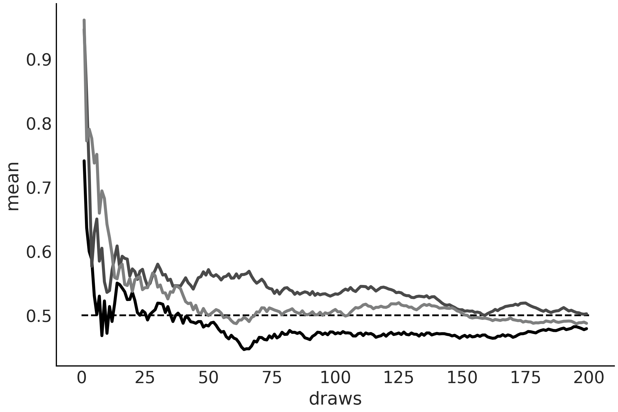
Fig. 11.18 Running values from a \(\mathcal{U}(0, 1)\) distribution. The dashed line at 0.5 represent the expected value. As the number of draws increases, the empirical mean approaches the expected value. Each line represents a different sample.#
11.1.10.2. The Central Limit Theorem#
The central limit theorem states that if we sample \(n\) values independently from an arbitrary distribution the mean \(\bar X\) of those values will distribute approximately as a Gaussian as \({n \rightarrow \infty}\):
where \(\mu\) and \(\sigma^2\) are the mean and variance of the arbitrary distribution.
For the central limit theorem to be fulfilled, the following assumptions must be met:
The values are sampled independently
Each value come from the same distribution
The mean and standard deviation of the distribution must be finite
Criteria 1 and 2 can be relaxed quite a bit and we will still get roughly a Gaussian, but there is no way to escape from Criterion 3. For distributions such as the Cauchy distribution, which do not have a defined mean or variance, this theorem does not apply. The average of \(N\) values from a Cauchy distribution do not follow a Gaussian but a Cauchy distribution.
The central limit theorem explains the prevalence of the Gaussian distribution in nature. Many of the phenomena we study can be explained as fluctuations around a mean, or as the result of the sum of many different factors.
Fig. 11.19 shows the central limit theorem in action for 3 different distributions, \(\text{Pois}(2.3)\), \(\mathcal{U}(0, 1)\), \(\text{Beta}(1, 10)\), as \(n\) increases.
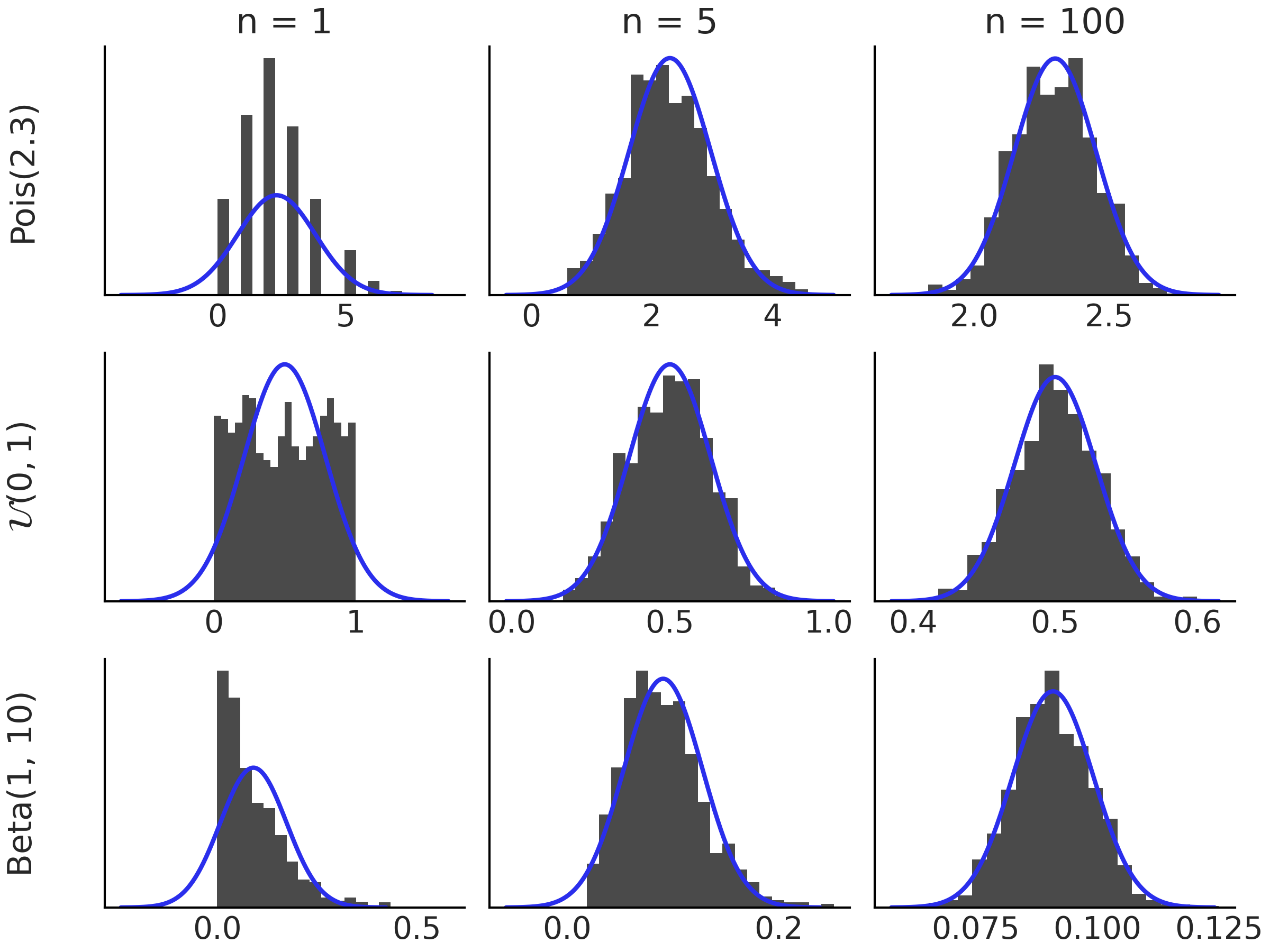
Fig. 11.19 Histograms of the distributions indicated on the left margin. Each histogram is based on 1000 simulated values of \(\bar{X_n}\). As we increase \(n\) the distribution of \(\bar{X_n}\) approach a Normal distribution. The black curve corresponds to a Gaussian distribution according to the central limit theorem.#
11.1.11. Markov Chains#
A Markov Chain is a sequence of random variables \(X_0, X_1, \dots\) for which the future state is conditionally independent from all past ones given the current state. In other words, knowing the current state is enough to know the probabilities for all future states. This is known as the Markov property and we can write it as:
A rather effective way to visualize Markov Chains is imagining you or some object moving in space [15]. The analogy is easier to grasp if the space is finite, for example, moving a piece in a square board like checkers or a salesperson visiting different cities. Given this scenarios you can ask questions like, how likely is to visit one state (specific squares in the board, cities, etc)? Or maybe more interesting if we keep moving from state to state how much time will we spend at each state in the long-run?
Fig. 11.20 shows four examples of Markov Chains, the first one show a classical example, an oversimplified weather model, where the states are rainy or sunny, the second example shows a deterministic die. The last two example are more abstract as we have not assigned any concrete representation to them.
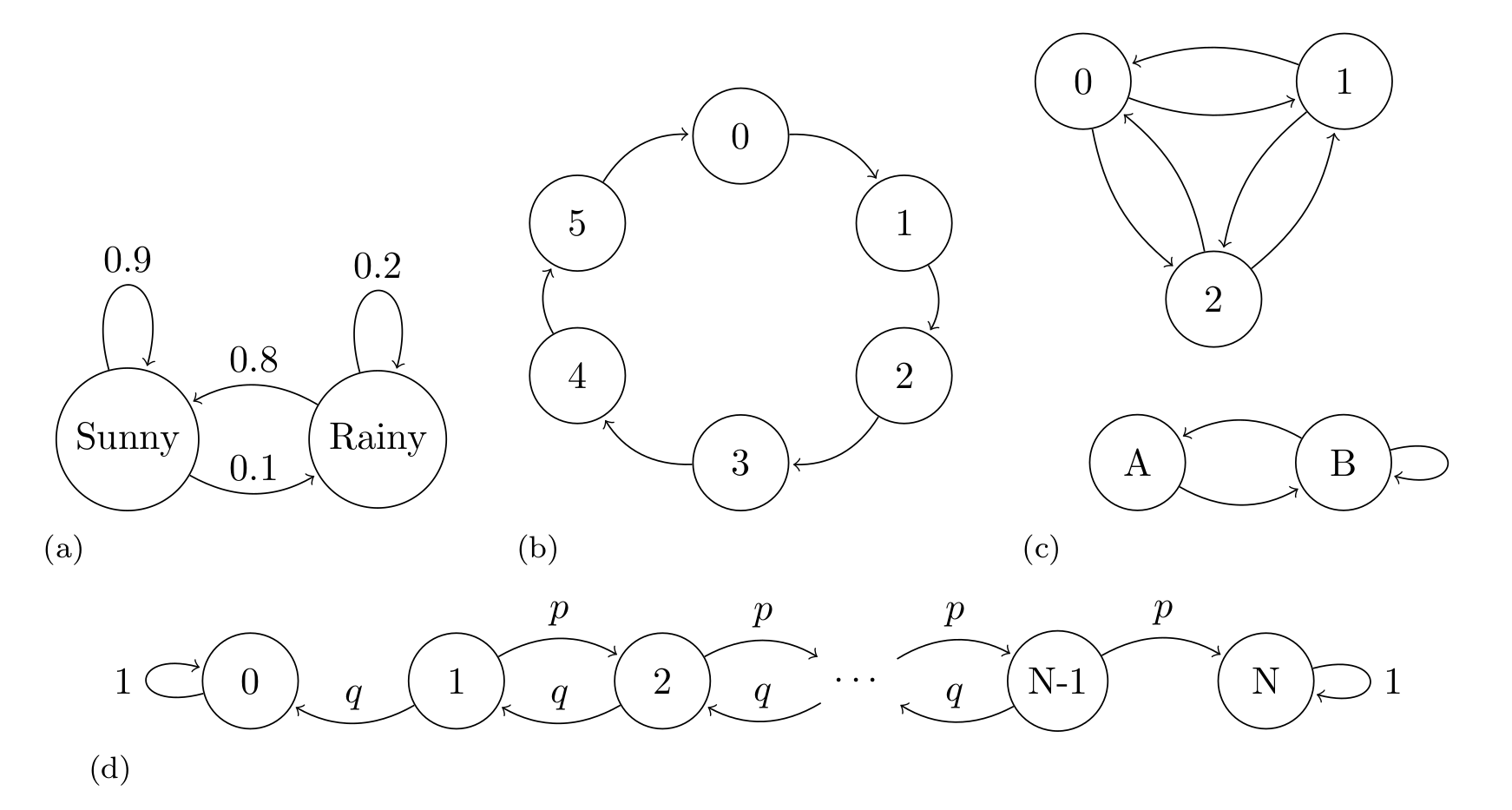
Fig. 11.20 Markov Chains examples. (a) An oversimplified weather model, representing the probability of a rainy or sunny day, the arrows indicate the transition between states, the arrows are annotated with their corresponding transition probabilities. (b) An example of periodic Markov Chain. (c) An example of a disjoint chain. The states 1, 2, and 3 are disjoint from states A and B. If we start at the state 1, 2, or 3 we will never reach state A or B and vice versa. Transition probabilities are omitted in this example. (d) A Markov chain representing the gambler’s ruin problem, two gamblers, A and B, start with \(i\) and \(N-i\) units of money respectively. At any given money they bet 1 unit, gambler A has probability \(p\) of and probability \(q = 1 - p\) of losing. If \(X_n\) is the total money of gambler A at time \(n\). Then \(X_0, X_1, \dots\) is a Markov chain as the one represented.#
A convenient way to study Markov Chains is to collect the probabilities of moving between states in one step in a transition matrix \(\mathbf{T} = (t_{ij})\). For example, the transition matrix of example A in Fig. 11.20 is
and, for example, the transition matrix of example B in Fig. 11.20 is
The \(i\)th row of the transition matrix represents the conditional probability distribution of moving from state \(X_{n}\) to the state \(X_{n+1}\). That is, \(p(X_{n+1} \mid X_n = i)\). For example, if we are at state sunny we can move to sunny (i.e. stay at the same state) with probability 0.9 and move to state rainy with probability 0.1. Notice how the total probability of moving from sunny to somewhere is 1, as expected for a PMF.
Because of the Markov property we can compute the probability of \(n\) consecutive steps by taking the \(n\)th power of \(\mathbf{T}\).
We can also specify the starting point of the Markov chain, i.e. the initial conditions \(s_i = P(X_0 = i)\) and let \(\mathbf{s}=(s_1, \dots, s_M)\). With this information we can compute the marginal PMF of \(X_n\) as \(\mathbf{s}\mathbf{T}^n\).
When studying Markov chains it makes sense to define properties of individual states and also properties on the entire chain. For example, if a chain returns to a state over and over again we call that state recurrent. Instead a transient state is one that the chain will eventually leave forever, in example (d) in Fig. 11.20 all states other than 0 or \(N\) are transient. Also, we can call a chain irreducible if it is possible to get from any state to any other state in a finite number of steps example (c) in Fig. 11.20 is not irreducible, as states 1,2 and 3 are disconnected from states A and B.
Understanding the long-term behavior of Markov chains is of interest. In fact, they were introduced by Andrey Markov with the purpose of demonstrating that the law of large numbers can be applied also to non-independent random variables. The previously mentioned concepts of recurrence and transience are important for understanding this long-term run behavior. If we have a chain with transient and recurrent states, the chain may spend time in the transient states, but it will eventually spend all the eternity in the recurrent states. A natural question we can ask is how much time the chain is going to be at each state. The answer is provided by finding the stationary distribution of the chain.
For a finite Markov chain, the stationary distribution \(\mathbf{s}\) is a PMF such that \(\mathbf{s}\mathbf{T} = \mathbf{s}\) [16]. That is a distribution that is not changed by the transition matrix \(\mathbf{T}\). Notice that this does not mean the chain is not moving anymore, it means that the chain moves in such a way that the time it will spend at each state is the one defined by \(\mathbf{s}\). Maybe a physical analogy could helps here. Imagine we have a glass not completely filled with water at a given temperature. If we seal it with a cover, the water molecules will evaporate into the air as moisture. Interestingly it is also the case that the water molecules in the air will move to the liquid water. Initially more molecules might be going one way or another, but at a given point the system will find a dynamic equilibrium, with the same amount of water molecules moving to the air from the liquid water, as the number of water molecules moving from the liquid water to the air. In physics/chemistry this is called a steady-state, locally things are moving, but globally nothing changes [17]. Steady state is also an alternative name to stationary distribution.
Interestingly, under various conditions, the stationary distribution of a finite Markov chain exists and is unique, and the PMF of \(X_n\) converges to \(\mathbf{s}\) as \(n \to \infty\). Example (d) in Fig. 11.20 does not have a unique stationary distribution. We notice that once this chain reaches the states 0 or \(N\), meaning gambler A or B lost all the money, the chain stays in that state forever, so both \(s_0=(1, 0, \dots , 0)\) and \(s_N=(0, 0, \dots , 1)\) are both stationary distributions. On the contrary example B in Fig. 11.20 has a unique stationary distribution which is \(s=(1/6, 1/6, 1/6, 1/6, 1/6, 1/6)\), event thought the transition is deterministic.
If a PMF \(\mathbf{s}\) satisfies the reversibility condition (also known as detailed balance), that is \(s_i t_{ij} = s_j t_{ji}\) for all \(i\) and \(j\), we have the guarantee that \(\mathbf{s}\) is a stationary distribution of the Markov chain with transition matrix \(\mathbf{T} = t_{ij}\). Such Markov chains are called reversible. In Section Inference Methods we will use this property to show why Metropolis-Hastings is guaranteed to, asymptotically, work.
Markov chains satisfy a central limit theorem which is similar to Equation (11.34) except that instead of dividing by \(n\) we need to divide by the effective sample size (ESS). In Section Effective Sample Size we discussed how to estimate the effective sample size from a Markov Chain and how to use it to diagnose the quality of the chain. The square root of \(\frac{\sigma^2} {\text{ESS}}\) is the Monte Carlo standard error (MCSE) that we also discussed in Section Monte Carlo Standard Error.
11.2. Entropy#
In the Zentralfriedhof, Vienna, we can find the grave of Ludwig Boltzmann. His tombstone has the legend \(S = k \log W\), which is a beautiful way of saying that the second law of thermodynamics is a consequence of the laws of probability. With this equation Boltzmann contributed to the development of one of the pillars of modern physics, statistical mechanics. Statistical mechanics describes how macroscopic observations such as temperature are related to the microscopic world of molecules. Imagine a glass with water, what we perceive with our senses is basically the average behavior of a huge number water molecules inside that glass [18]. At a given temperature there is a given number of arrangements of the water molecules compatible with that temperature (Figure Fig. 11.21). As we decrease the temperature we will find that less and less arrangements are possible until we find a single one. We have just reached 0 Kelvin, the lowest possible temperature in the universe! If we move into the other direction we will find that molecules can be found in more and more arrangements.
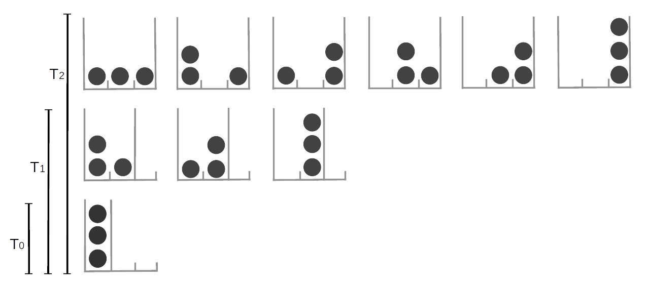
Fig. 11.21 The number of possible arrangements particles can take is related to the temperature of the system. Here we represent discrete system of 3 equivalent particles, the number of possible arrangements is represented by the available cells (gray high lines). increasing the temperature is equivalent to increasing the number of available cells. At \(T=0\) only one arrangement is possible, as the temperature increase the particles can occupy more and more states.#
We can analyze this mental experiment in terms of uncertainty. If we know a system is at 0 Kelvin we know the system can only be in a single possible arrangement, our certainty is absolute [19], as we increase the temperature the number of possible arrangements will increase and then it will become more and more difficult to say, “Hey look! Water molecules are in this particular arrangement at this particular time!” Thus our uncertainty about the microscopic state will increase. We will still be able to characterize the system by averages such the temperature, volume, etc, but at the microscopic level the certainty about particular arrangements will decrease. Thus, we can think of entropy as a way of measuring uncertainty.
The concept of entropy is not only valid for molecules. It could also be applies to arrangements of pixels, characters in a text, musical notes, socks, bubbles in a sourdough bread and more. The reason that entropy is so flexible is because it quantifies the arrangements of objects - it is a property of the underlying distributions. The larger the entropy of a distribution the less informative that distribution will be and the more evenly it will assign probabilities to its events. Getting an answer of “\(42\)” is more certain than “\(42 \pm 5\)”, which again more certain than “any real number”. Entropy can translate this qualitative observation into numbers.
The concept of entropy applies to continue and discrete distributions, but it is easier to think about it using discrete states and we will see some example in the rest of this section. But keep in mind the same concepts apply to the continuous cases.
For a probability distribution \(p\) with \(n\) possible different events which each possible event \(i\) having probability \(p_i\), the entropy is defined as:
Equation (11.36) is just a different way of writing the entropy engraved on Boltzmann’s tombstone. We annotate entropy using \(H\) instead of \(S\) and set \(k=1\). Notice that the multiplicity \(W\) from Boltzmann’s version is the total number of ways in which different outcomes can possibly occur:
You can think of this as rolling a t-sided die \(N\) times, where \(n_i\) is the number of times we obtain side \(i\). As \(N\) is large we can use Stirling’s approximation \(x! \approx (\frac{x}{e})^x\).
noticing that \(p_i = \frac{n_i}{N}\) we can write:
And finally by taking the logarithm we obtain
which is exactly the definition of entropy.
We will now show how to compute entropy in Python using Code Block entropy_dist, with the result shown in Fig. 11.22.
x = range(0, 26)
q_pmf = stats.binom(10, 0.75).pmf(x)
qu_pmf = stats.randint(0, np.max(np.nonzero(q_pmf))+1).pmf(x)
r_pmf = (q_pmf + np.roll(q_pmf, 12)) / 2
ru_pmf = stats.randint(0, np.max(np.nonzero(r_pmf))+1).pmf(x)
s_pmf = (q_pmf + np.roll(q_pmf, 15)) / 2
su_pmf = (qu_pmf + np.roll(qu_pmf, 15)) / 2

_, ax = plt.subplots(3, 2, figsize=(12, 5), sharex=True, sharey=True,
                     constrained_layout=True)
ax = np.ravel(ax)

zipped = zip([q_pmf, qu_pmf, r_pmf, ru_pmf, s_pmf, su_pmf],
             ["q", "qu", "r", "ru", "s", "su"])
for idx, (dist, label) in enumerate(zipped):
    ax[idx].vlines(x, 0, dist, label=f"H = {stats.entropy(dist):.2f}")
    ax[idx].set_title(label)
    ax[idx].legend(loc=1, handlelength=0)
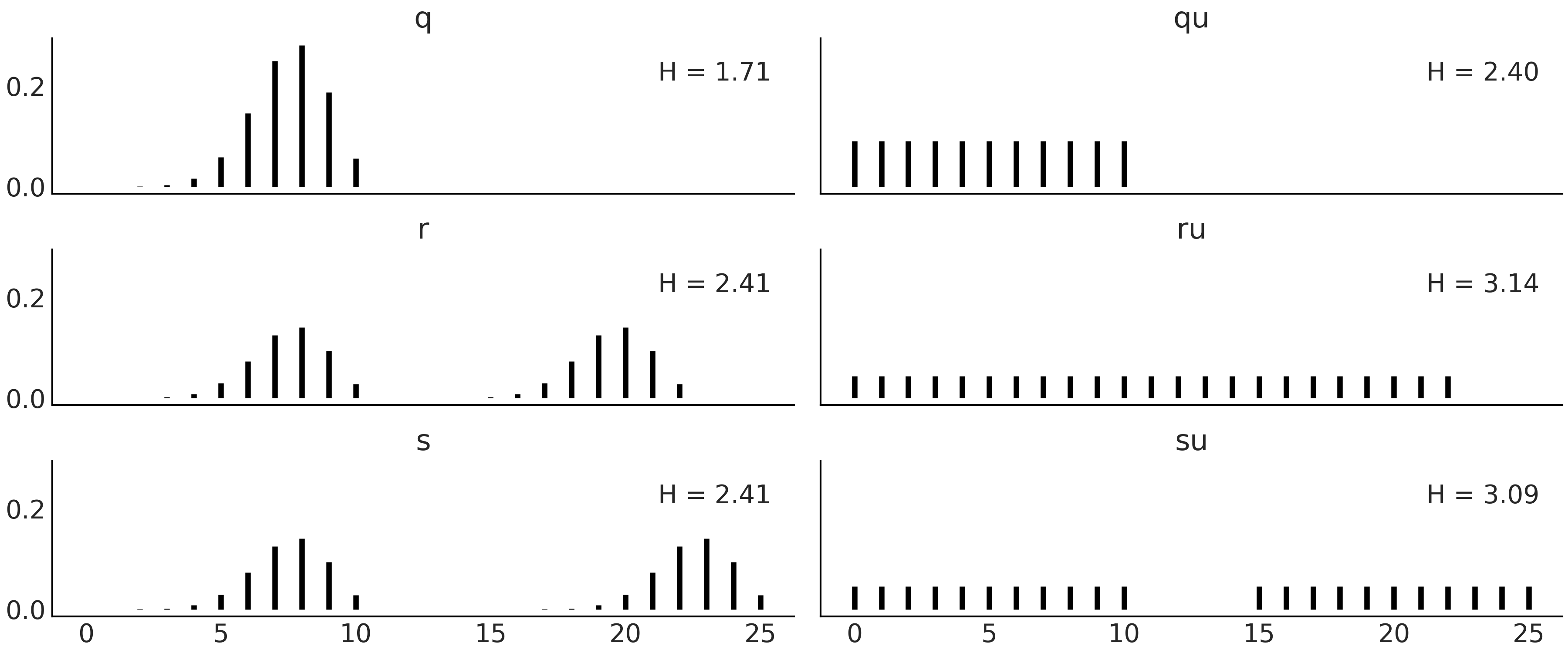
Fig. 11.22 Discrete distributions defined in Code Block entropy_dist and their entropy values \(H\).#
Fig. 11.22 shows six distributions, one per subplot with its corresponding entropy. There are a lot of things moving on in this figure, so before diving in be sure to set aside an adequate amount of time (this maybe a good time to check your e-mails before going on). The most peaked, or least spread distribution is \(q\), and this is the distribution with the lowest value of entropy among the six plotted distributions. \(q \sim \text{binom}({n=10, p=0.75})\), and thus there are 11 possible events. \(qu\) is a Uniform distribution with also 11 possible events. We can see that the entropy of \(qu\) is larger than \(q\), in fact we can compute the entropy for binomial distributions with \(n=10\) and different values of \(p\) and we will see that none of them have larger entropy than \(qu\). We will need to increase \(n\) \(\approx 3\) times to find the first binomial distribution with larger entropy than \(qu\). Let us move to the next row. We generate distribution \(r\) by taking \(q\) and shifting it to the right and then normalizing (to ensure the sum of all probabilities is 1). As \(r\) is more spread than \(q\) its entropy is larger. \(ru\) is the Uniform distribution with the same number of possible events as \(r\) (22), notice we are including as possible values those in the valley between both peaks. Once again the entropy of the Uniform version is the one with the largest entropy. So far entropy seems to be proportional to the variance of a distribution, but before jumping to conclusions let us check the last two distributions in Fig. 11.22. \(s\) is essentially the same as \(r\) but with a more extensive valley between both peaks and as we can see the entropy remains the same. The reason is basically that entropy does not care about those events in the valley with probability zero, it only cares about possible events. \(su\) is constructed by replacing the two peaks in \(s\) with \(qu\) (and normalizing). We can see that \(su\) has lower entropy than \(ru\) even when it looks more spread, after a more careful inspection we can see that \(su\) spread the total probability between fewer events (22) than \(ru\) (with 23 events), and thus it makes totally sense for it to have lower entropy.
11.3. Kullback-Leibler Divergence#
It is common in statistics to use one probability distribution \(q\) to represent another one \(p\), we generally do this when we do not know \(p\) but can approximate it with \(q\). Or maybe \(p\) is complex and we want to find a simpler or more convenient distribution \(q\). In such cases we may ask how much information are we losing by using \(q\) to represent \(p\), or equivalently how much extra uncertainty are we introducing. Intuitively, we want a quantity that becomes zero only when \(q\) is equal to \(p\) and be a positive value otherwise. Following the definition of entropy in Equation (11.36), we can achieve this by computing the expected value of the difference between \(\log(p)\) and \(\log(q)\). This is known as the Kullback-Leibler (KL) divergence:
Thus the \(\mathbb{KL}(p \parallel q)\) give us the average difference in log probabilities when using \(q\) to approximate \(p\). Because the events appears to us according to \(p\) we need to compute the expectation with respect to \(p\). For discrete distributions we have:
Using logarithmic properties we can write this into probably the most common way to represent KL divergence:
We can also arrange the term and write the \(\mathbb{KL}(p \parallel q)\) as:
and when we expand the above rearrangement we find that:
As we already saw in previous section, \(H(p)\) is the entropy of \(p\). \(H(p,q) = - \mathbb{E}_p[\log{q}]\) is like the entropy of \(q\) but evaluated according to the values of \(p\).
Reordering above we obtain:
This shows that the KL divergences can be effectively interpreted as the extra entropy with respect to \(H(p)\), when using \(q\) to represent \(p\).
To gain a little bit of intuition we are going to compute a few values for the KL divergence and plot them., We are going to use the same distributions as in Fig. 11.22.
dists = [q_pmf, qu_pmf, r_pmf, ru_pmf, s_pmf, su_pmf]
names = ["q", "qu", "r", "ru", "s", "su"]

fig, ax = plt.subplots()
KL_matrix = np.zeros((6, 6))
for i, dist_i in enumerate(dists):
    for j, dist_j in enumerate(dists):
        KL_matrix[i, j] = stats.entropy(dist_i, dist_j)

im = ax.imshow(KL_matrix, cmap="cet_gray")
The result of Code Block kl_varies_dist is shown in Fig. 11.23. There are two features of Fig. 11.23 that immediately pop out. First, the figure is not symmetric, the reason is that \(\mathbb{KL}(p \parallel q)\) is not necessarily the same as \(\mathbb{KL}(q \parallel p)\). Second, we have many white cells. They represent \(\infty\) values. The definition of the KL divergence uses the following conventions [134]:
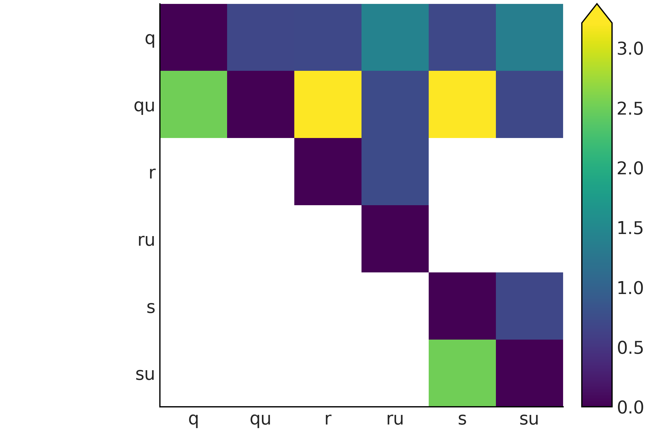
Fig. 11.23 KL divergence for all the pairwise combinations of the distributions q, qu, r, ru, s, and su shown in Fig. 11.22, the white color is used to represent infinity values.#
We can motivate the use of a log-score in computing expected log pointwise predictive density (introduced in Chapter 2 Equation (2.5)) based on the KL divergence. Let us assume we have \(k\) models posteriors \(\{q_{M_1}, q_{M_2}, \cdots q_{M_k}\}\), let further assume we know the true model \(M_0\) then we can compute:
This may seems a futile exercise as in real life we do not know the true model \(M_0\). The trick is to realize that as \(p_{M_0}\) is the same for all comparisons, thus building a ranking based on the KL-divergence is equivalent to doing one based on the log-score.
11.4. Information Criterion#
An information criterion is a measure of the predictive accuracy of a statistical model. It takes into account how well the model fits the data and penalizes the complexity of the model. There are many different information criterion based on how they compute these two terms. The most famous family member, especially for non-Bayesians, is the Akaike Information Criterion (AIC) [135]. It is defined as the sum of two terms. The \(\log p(y_i \mid \hat{\theta}_{mle})\) measures how well the model fits the data and the penalization term \(p_{AIC}\) to account for the fact that we use the same data to fit the model and to evaluate the model.
where \(\hat{\theta}_{mle}\) is the maximum-likelihood estimation of \(\boldsymbol{\theta}\) and \(p_{AIC}\) is just the number of parameters in the model.
AIC is quite popular in non-Bayesian settings, but is not well equipped to deal with the generality of Bayesian models. It does not use the full posterior distribution, thus discarding potentially useful information. On average, AIC will behave worse and worse as we move from flat prior into weakly-informative or informative priors, and/or if we add more structure into our model, like with hierarchical models. AIC assumes that the posterior can be well represented (at least asymptotically) by a Gaussian distribution, but this is not true for a number of models, including hierarchical models, mixture models, neural networks, etc. In summary we want to use some better alternatives.
The Widely applicable Information Crieria (WAIC [20]) [136] can be regarded as a fully Bayesian extension of AIC. It also contains two terms, roughly with the same interpretation as the Akaike criterion. The most important difference is that the terms are computed using the full posterior distribution.
The first term in Equation (11.50) is just the log-likelihood as in AIC but evaluated pointwise, i.e, at each \(i\) observed data-point over the \(n\) observations. We are taking into account the uncertainty in the posterior by taking the average over the \(s\) samples from the posterior. This first term is a practical way to compute the theoretical expected log pointwise predictive density (ELPD) as defined in Equation (2.4) and its approximation in Equation (2.5).
The second term might look a little bit weird, as is the variance over the \(s\) posterior samples (per observation). Intuitively, we can see that for each observation the variance will be low if the log-likelihood across the posterior distribution is similar and it will be larger if the log-likelihood varies more for different samples from the posterior distribution. The more observations we find to be sensitive to the details of the posterior the larger the penalization will be. We can also see this from another equivalent perspective; A more flexible model is one that can effectively accommodate more datasets. For example, a model that included straight but also upward curves is more flexible than one that only allows straight lines; and thus the log-likelihood of those observation evaluated across the posterior on the later model will have, on average, a higher variance. If the more flexible model is not able to compensate this penalization with a higher estimated ELPD then the simpler model will we ranked as a better choice. Thus the variance term in Equation (11.50) prevents overfitting by penalizing an overly complex model and it can be loosely interpreted as the effective number of parameters as in AIC.
Neither AIC nor WAIC are attempting to measure whether the model is true, they are only a relative measure to compare alternative models. From a Bayesian perspective the prior is part of the model, but WAIC is evaluated over the posterior, and the prior effect is only indirectly taken into account by the way it affects the resulting posterior. There are other information criteria like BIC and WBIC that attempts to answer that question and can be seen as approximations to the Marginal Likelihood, but we do not discuss them in this book.
11.5. LOO in Depth#
As discussed in Section Cross-validation and LOO in this book we use the term LOO to refer to a particular method to approximate Leave-One-Out Cross-Validation (LOO-CV) known as Pareto Smooth Importance Sampling Leave Once Out Cross Validation (PSIS-LOO-CV). In this section we are going to discuss a few details of this method.
LOO is an alternative to WAIC, in fact it can be shown that asymptotically they converge to the same numerical value [136, 137]. Nevertheless, LOO presents two importance advantages for practitioners. It is more robust in finite samples settings, and it provides useful diagnostics during computation [16, 137].
Under LOO-CV the expected log pointwise predictive density for a new dataset is:
where \(y_{-i}\) represents the dataset excluding the \(i\) observation.
Given that in practice we do not know the value of \(\boldsymbol{\theta}\) we can approximate Equation \(\ref{eq:elpd_loo_cv}\) using \(s\) samples from the posterior:
Notice that this term looks similar to the first term in Equation (11.50), except we are computing \(n\) posteriors removing one observation each time. For this reason, and contrary to WAIC, we do not need to add a penalization term. Computing \(\text{ELPD}_\text{LOO-CV}\) in (11.51) is very costly as we need to compute \(n\) posteriors. Fortunately if the \(n\) observations are conditionally independent we can approximate Equation (11.51) with Equation (11.52) [137, 138]:
where \(w\) is a vector of normalized weights.
To compute \(w\) we used importance sampling, this is a technique for estimating properties of a particular distribution \(f\) of interest, given that we only have samples from a different distribution \(g\). Using importance sampling makes sense when sampling from \(g\) is easier than sampling from \(f\). If we have a set of samples from the random variable \(X\) and we are able to evaluate \(g\) and \(f\) pointwise, we can compute the importance weights as:
Computationally, it goes as follow:
Draw \(N\) samples \(x_i\) from \(g\)
Calculate the probability of each sample \(g(x_i)\)
Evaluate \(f\) over the \(N\) samples \(f(x_i)\)
Calculate the importance weights \(w_i = \frac{f(x_i)}{g(x_i)}\)
Return \(N\) samples from \(g\) with weights \(w\), \((x_i, w_i)\), that could be plug into some estimator
Fig. 11.24 shows an example of approximating the same target distribution (dashed line) by using two different proposal distributions. On the first row the proposal is wider than the target distribution. On the second row the proposal is narrower than the target distribution. As we can see the approximation is better in the first case. This is a general feature of importance sampling.
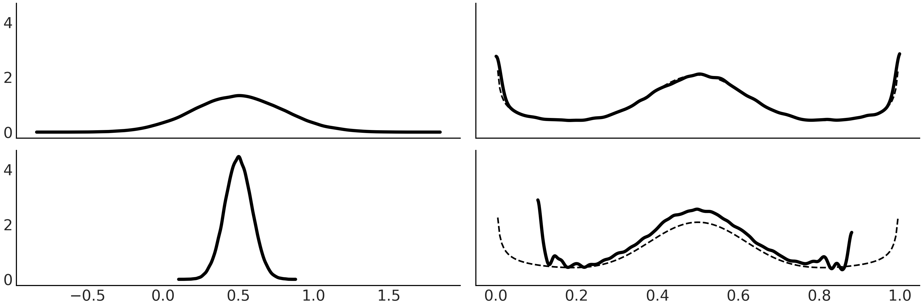
Fig. 11.24 Importance sampling. On the left we have KDEs of samples from the proposal distributions \(g\), on the right the dashed line represents the target distribution and the continuous line the approximated distribution after re-weighting the samples from the proposal distribution with the weights computed as in Equation (11.53).#
Going back to LOO, the distribution that we have computed is the posterior distribution. In order to evaluate the model we want samples from the leave-one-out posterior distribution, thus the importance weights we want to compute are:
Notice that this proportionality is great news, because it allows us to compute \(w\) almost for free. However, the posterior is likely to have thinner tails than the leave-one-out distributions, which as we saw in Fig. 11.24 can result in poor estimation. Mathematically the problem is that the importance weights can have high or even infinite variance. In order to keep the variance in check, LOO applies a smoothing procedure that involves replacing the largest importance weights with values from an estimated Pareto distribution. This help to make LOO much more robust [137]. Moreover, the estimated \(\hat \kappa\) parameter of the Pareto distribution can be used to detect highly influential observations, i.e. observations that have a large effect on the predictive distribution when they are left out. In general, higher values of \(\hat \kappa\) can indicate problems with the data or model, especially when \(\hat \kappa > 0.7\) [16, 22].
11.6. Jeffreys’ Prior Derivation#
In this section we will show how to find the Jeffreys’ prior for the binomial likelihood, first for the number of successes parameter \(\theta\), and then for the odds parameter \(\kappa\), where \(\kappa = \frac{\theta}{1-\theta}\).
Recall from Chapter 1, for the one-dimensional case JP for \(\theta\) is defined as:
where \(I(\theta)\) is the Fisher information:
11.6.1. Jeffreys’ Prior for the Binomial Likelihood in Terms of \(\theta\)#
Binomial likelihood could be expressed as:
where \(y\) is the number of successes, \(n\) the total number of trials, and thus \(n-y\) is the numbers of failures. We write is as a proportionality as the Binomial coefficient in the likelihood does not depend on \(\theta\).
To compute the Fisher information we need to take the logarithm of the likelihood:
And then compute the second derivative:
The Fisher information is the expected value of the second derivative of the likelihood, then:
As \(\mathbb{E}[y] = n\theta\), we can write:
which we can rewrite as:
We can express these fractions in terms of a common denominator,
By regrouping:
If we omit \(n\) then we can write:
Finally, we need to take the square root of the Fisher information in Equation (11.63), which resulting the Jeffreys’ prior for \(\theta\) of Binomial likelihood as follow:
11.6.2. Jeffreys’ Prior for the Binomial Likelihood in Terms of \(\kappa\)#
Let us now see how to obtain the Jeffreys’ prior for the Binomial likelihood in terms the odds \(\kappa\). We begin by replacing \(\theta = \frac{\kappa}{\kappa + 1}\) in expression (11.55):
Which can also be written as:
and further simplified into:
Now we need to take the logarithm:
we then compute the second derivative:
The Fisher information is the expected value of the second derivative of the likelihood, then:
As \(\mathbb{E}[y] = n \theta = n \frac{\kappa}{\kappa + 1}\), we can write:
We can express these fractions in terms of a common denominator,
Then we combine into a single fraction
We then distribute \(n\) over \((\kappa + 1)\) and we simplify:
Finally, by taking the square root, we get the Jeffreys’ prior for the Binomial likelihood when parameterized by the odds:
11.6.3. Jeffreys’ Posterior for the Binomial Likelihood#
To obtain the Jeffrey’s posterior when the likelihood is parameterized in terms of \(\theta\) we can combine Equation (11.55) with Equation (11.64)
Similarly, the Jeffreys’ posterior when the likelihood is parameterized in terms of \(\kappa\) we can combine (11.67) with (11.75)
11.7. Marginal Likelihood#
For some models, such as those using conjugate priors, the marginal likelihood is analytically tractable. For the rest, numerically computing this integral is notoriously difficult, since this involves a high-dimensional integration over a usually complicated and highly variable function [139]. In this section we will try to gain intuition into why this is generally a hard task.
Numerically, and in low dimensions, we can compute the marginal likelihood by evaluating the product of the prior and the likelihood, over a grid and then applying the trapezoid rule, or some other similar method. As we will see in Section Moving out of Flatland using grids does not scale well with dimension, as the number of required grid points increase rapidly as we increase the number of variables in our model. Thus grid-based methods becomes impractical for problems with more than a few variables. Monte Carlo integration can also be problematic, at least in the most naive implementations (see Section Moving out of Flatland). For that reason many dedicated methods have been proposed to compute the marginal likelihood [139]. Here we will only discuss one of them. Our main concern is not learning how to compute the marginal likelihood in practice, but instead to illustrate why is hard to do it.
11.7.1. The Harmonic Mean Estimator#
A rather infamous estimator of the marginal likelihood is the harmonic mean estimator [140]. A very appealing feature of this estimator is that it only requires \(s\) samples from the posterior:
We can see that we are averaging the inverse of the likelihood over samples taken from the posterior, then computing the inverse of the result. In principle, this is a valid Monte Carlo estimator of the following expectation:
Notice that Equation (11.79) is a particular instance of Equation (1.5) which may seems to indicate we are doing something right by being very Bayesian.
If we expand the posterior term we can write:
which we can simplify into:
We are assuming the prior is proper, and thus its integral should be 1. We can see that Equation (11.78) is in fact an approximation of the marginal likelihood.
Unfortunately the good news does not last too long. The number of samples \(s\) needed to feed into Equation (11.78) in order to get close to the right answer is generally very large, to the point that the harmonic mean estimator is not very useful in practice [139, 140]. Intuitively we can see that the sum will be dominated by samples with very low likelihood. Even worse, the harmonic mean estimator can have infinite variance. Infinite variance means that even if we increase \(s\) we will not get a better answer, thus sometimes even a huge amount of samples could still be insufficient. The other problem with the harmonic mean estimator is that it is rather insensitive to changes in the prior. But even the exact marginal likelihood is in fact very sensitive to changes in the prior distribution (as we will show later, see Fig. 11.26). These two problems will be exacerbated when the likelihood turns to be much more concentrated with respect to the prior, or when the likelihood and prior concentrate into different regions of the parameter space.
By using samples from a more peaked posterior, with respect to the prior, we will be missing all the regions from the prior that have low posterior density. In a sketchy way we can think of Bayesian Inference as using data to update the prior into a posterior. Prior and posterior will only be similar if the data is not very informative.
Fig. 11.25 shows a heatmap with the relative error of computing the harmonic mean estimator compared to the analytical value. We can see than even for a simple 1D problem like the Beta-Binomial model the harmonic estimator can fail spectacularly.
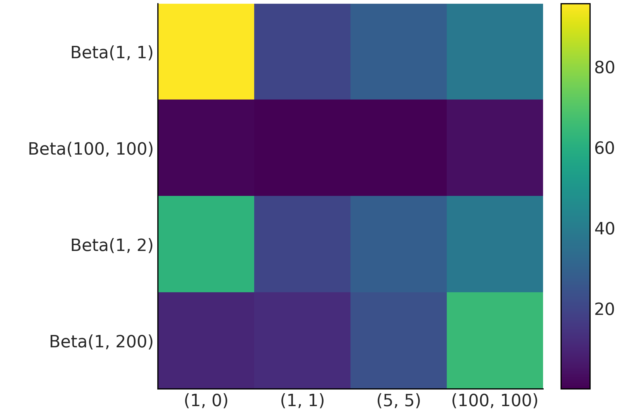
Fig. 11.25 Heatmap showing the relative error when using the harmonic mean estimator to approximate the marginal likelihood of a Beta-Binomial model. Rows corresponds to different prior distributions. Each column is a different observed scenario, with the number in parentheses corresponding to the number of success and failures.#
As we will see in Section Moving out of Flatland when we increase the dimensionality of our models the posterior concentrates more an more into a thin hyper-shell. Getting samples from outside this thin shell is irrelevant to compute a good posterior approximation. On the contrary when computing the marginal likelihood obtaining samples just from this thin shell is not enough. Instead, we need to take samples over the entire prior distribution and this can be a really hard task to do in a proper way.
There are a few computational methods better suited to compute marginal likelihood, but even those are not bullet-proof. In Chapter 8 we discuss the Sequential Monte Carlo (SMC) method mainly for the purpose of doing Approximate Bayesian Computation, but this method can also compute the marginal likelihood. The main reason why it works is because SMC uses a series of intermediate distributions to represent the transition from the prior to the posterior distributions. Having these bridging distribution alleviates the problem of sampling from a wide prior and evaluating in a much more concentrated posterior.
11.7.2. Marginal Likelihood and Model Comparison#
When performing inference the marginal likelihood is generally regarded as a normalization constant and often could be omitted or canceled out during computation. Instead, the marginal likelihood is often seen as crucial during model comparison [141, 142, 143]. To better understand why let us write Bayes’ theorem in a way that explicitly shows that our inferences are model dependent:
where \(Y\) represents the data and \(\boldsymbol{\theta}\) represents the parameters in model \(M\).
If we have a set of \(k\) models and our main objective is to choose only one of them, we can choose the one with the largest value of the marginal likelihood \(p(Y \mid M)\). Choosing the model with the largest marginal likelihood is perfectly justified from Bayes theorem under the assumption of a discrete Uniform prior distribution for the \(k\) models under comparison.
If all models have the same a priori probability then computing \(p(Y \mid M)\) is equivalent to computing \(p(M \mid Y)\). Notice that we are talking about the prior probability we assign to models \(p(M)\) and not about the priors we assign to parameters for each model \(p(\theta \mid M)\).
As the value of \(p(Y \mid M_k)\) does not tell us anything by-itself, in practice people usually compute the ratio of two marginal likelihoods. This ratio is called Bayes factor:
Values of \(BF > 1\) indicates that model \(M_0\) it is better at explaining the data when compared with model \(M_1\). In practice it is common to use rules of thumb indicating when a BF is small, large, not that large, etc [21].
Bayes factor is appealing because it is a direct application of Bayes’ theorem as we can see from Equation (11.83), but this is also true for the harmonic mean estimator (see Section The Harmonic Mean Estimator) and that does not automatically makes it a good estimator. Bayes factor is also appealing because, contrary to the likelihood of a model, the marginal likelihood does not necessarily increases with the complexity of the model. The intuitive reason is that the larger the number of parameters the more spread out the prior will be with respect to the likelihood. Or in other words a more spread out prior is one that admits more datasets, as plausible, than a more concentrated one. This will be reflected in the marginal likelihood as we will get a smaller value with a wider prior than with a more concentrated prior.
Besides the computational problem, the marginal likelihood has a feature that it is usually considered as a bug. It is very sensitive to the choice of priors. By very sensitive we mean changes that while irrelevant for inference, have a practical effect in the value of the marginal likelihood. To exemplify this, assume we have the model:
The marginal log-likelihood for this model is can be computed analytically as follows:
σ_0 = 1
σ_1 = 1
y = np.array([0])
stats.norm.logpdf(loc=0, scale=(σ_0**2 + σ_1**2)**0.5, x=y).sum()
-1.2655121234846454
If you change the value of the prior parameter \(\sigma_0\) to 2.5 instead of 1, the marginal likelihood will be about 2 times smaller and by changing it to 10 it will be about 7 times smaller. You can use a PPL to compute the posterior for this model and see for yourself how influential is the change of the prior in the posterior. Additionally you can check Fig. 11.26 in the next section.
11.7.3. Bayes Factor vs WAIC and LOO#
In this book we do not use Bayes factors to compare model, we prefer instead the use of LOO. So it maybe useful to better understand how BFs are related to these other estimators. If we omit the details we can say that:
WAIC is the posterior-averaged log-likelihood
LOO is the posterior-averaged log-likelihood
The marginal likelihood is the prior-averaged (log)likelihood [22].
Let us discuss how this helps to understand the similarities and differences between these three quantities. All of them use a log-score as a measure of fitness with different computation. WAIC use a penalization term computed from the posterior variance. While both LOO and marginal likelihood avoids needing to use an explicit penalization term. LOO achieves this by approximating a leave-one-out cross-validation procedure. That is, it approximates using a dataset to fit the data and a different dataset to evaluate its fit. The penalization in marginal likelihood comes from averaging over the entire prior, with the spread of the prior (relatively) to the likelihood working as built-in penalizer. The penalization used in the marginal likelihood it seems to be somehow similar to the penalization in WAIC, although WAIC uses the variance of the posterior and so is close to the penalization in cross validation. Because, as previously discussed, a more spread prior admits more datasets as plausible than a more concentrated one, computing marginal likelihood is like implicitly averaging over all the datasets admitted by the prior.
An alternative, and equivalent, way to conceptualize the marginal likelihood is to notice that it is the prior predictive distribution evaluated at a particular dataset \(Y\). Thus, it is telling us how likely the data is under our model. And the model includes the prior and the likelihood.
For WAIC and LOO the role of the prior is indirect. The prior affects the value of WAIC and LOO only by its effect on the posterior. The more informative the data with respect to the prior, or in other words the greater the difference between prior and posterior, the less sensitive will be WAIC and LOO to the details of the prior. Instead, marginal likelihood use priors directly as we need to average the likelihood over the prior. Conceptually we can say that Bayes factors are focused on identifying the best model (and the prior is part of the model) while WAIC and LOO are focused on which (fitted) model and parameter will give the best predictions. Fig. 11.26 shows 3 posteriors for the model defined in Equation (11.85), for \(\sigma_0=1\), \(\sigma_0=10\) and \(\sigma_0=100\). As we can see, the posteriors are very close to each other, especially the last two. We can see that the values of WAIC and LOO only slightly change for the different posteriors, while the log marginal likelihood is sensitive to the choice of the prior. The posterior and log marginal likelihoods were computed analytically, WAIC and LOO were computed from samples from the posterior (for details see the accompanying code).
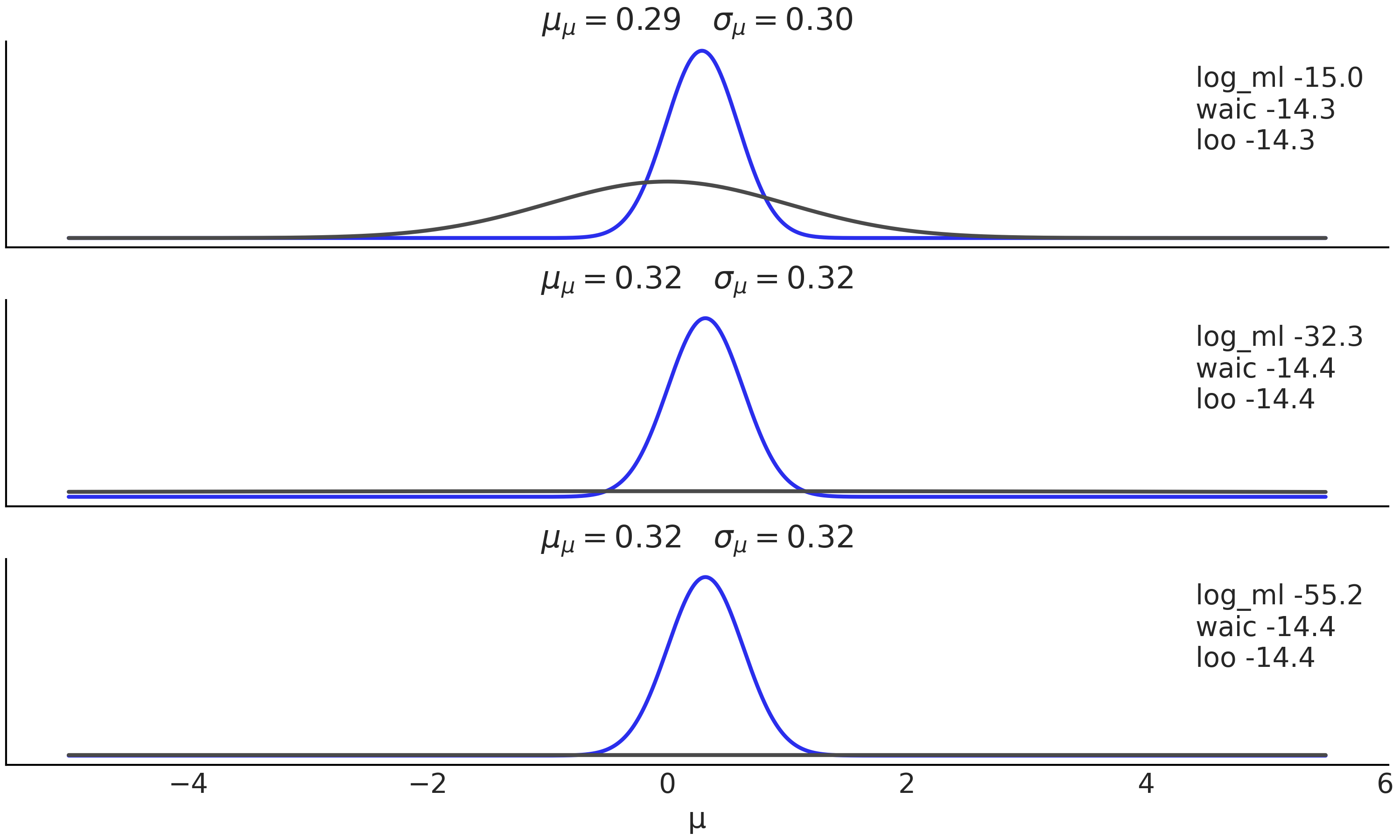
Fig. 11.26 Prior (gray line) and posterior (blue line) for the model in Equation (11.85). WAIC and LOO reflect that the posterior distributions are almost identical, while the marginal likelihood reflects that the prior are different.#
The above discussion helps to explain why Bayes factors are widely used in some fields and disliked in others. When priors are closer to reflecting some underlying true model, the sensitivity of the marginal likelihood to the prior specification is less worrisome. When priors are mainly used for their regularizing properties and when possible to provide some background knowledge, that sensitivity could be seen as problematic.
As a result, we think WAIC, and especially LOO, has more practical value, as their computation is generally more robust, and without the need to use special inference methods. And in the case of LOO, we also have good diagnostics.
11.8. Moving out of Flatland#
In Flatland: A Romance of Many Dimensions by Edwin Abbott [144] it tells the story of a square living in flatland, a two dimensional world inhabited by n-side polygons and where status is defined by the number of sides; with women being simple line-segments, and priests insisting they are circles even when then are just high-order polygons. The novel, first published in 1984, works equally well as social satire about the difficulties to understand ideas beyond our common experience.
As it happens to Square in flatland we are now going to evidence the weirdness of higher-dimensional spaces.
Suppose we want to estimate the value of \(\pi\). A simple procedure to do this is as follows. Inscribe a circle into a square, generate \(N\) points uniformly lying in that square and then count the proportion that fall inside the circle. Technically this is a Monte Carlo integration as we are calculating the value of a definite integral by using a (pseudo)random number generator.
The area of the circle and square are proportional to the number of points inside the circle and the total points. If the square has side \(2R\), it area will be \((2R)^2\) and the circle inscribe it inside of the square will have area \(\pi R^2\). The we have that:
By simplifying and rearranging we get that we can approximate \(\pi\) as:
We can implement this in a few lines of Python code as in Code Block montecarlo and the simulated points with the estimated value of \(\pi\) and the error of the approximation is shown in Fig. 11.27.
N = 10000
x, y = np.random.uniform(-1, 1, size=(2, N))
inside = (x**2 + y**2) <= 1
pi = inside.sum()*4/N
error = abs((pi - np.pi) / pi) * 100
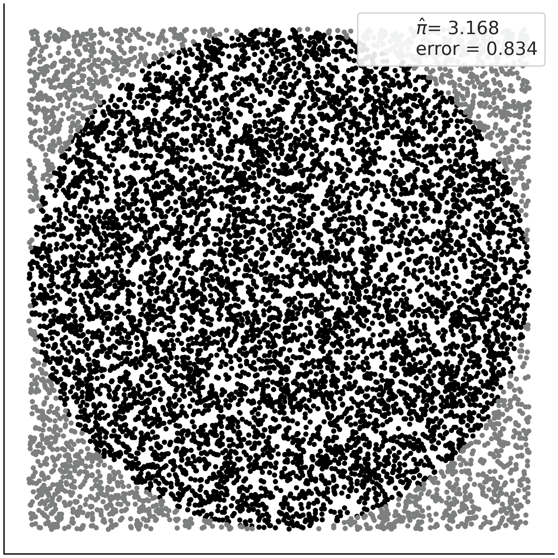
Fig. 11.27 Estimating \(\pi\) using Monte Carlo samples, legend shows the estimation and percentage error.#
As the draws are iid, we can apply the central limit theorem here and
then we know the error is reduced at a rate \(\frac{1}{\sqrt{N}}\)),
meaning that for each additional decimal place of accuracy we want we
will need to increase the number of draws N by a factor of 100.
What we have just done is an example of a Monte Carlo method [23], basically any method that uses (pseudo)random samples to compute something. And technically what we have done is a Monte Carlo integration as we are calculating the value of a definite integral (an area) by using samples. Monte Carlo methods are everywhere in statistics.
In Bayesian statistics we need to compute integrals to obtain posteriors or compute expectations from it. You may suggest that we can use a variation of this idea to compute quantities more interesting than \(\pi\). It turns out that this method will generally not work very well as we increase the dimensionality of the problem. In Code Block inside_out we count the number of points inside a circle when sampled from a square as we did before but from dimension 2 to 15. The result is in Fig. 11.28, weirdly, we see that as we increase the dimension of the problem and even when the hypersphere is touching the walls of the hypercube, the proportion of points inside drops rapidly. In a sense in higher dimensions all the volume of the hypercube is at the corners [24].
total = 100000

dims = []
prop = []
for d in range(2, 15):
    x = np.random.random(size=(d, total))
    inside = ((x * x).sum(axis=0) < 1).sum()
    dims.append(d)
    prop.append(inside / total)
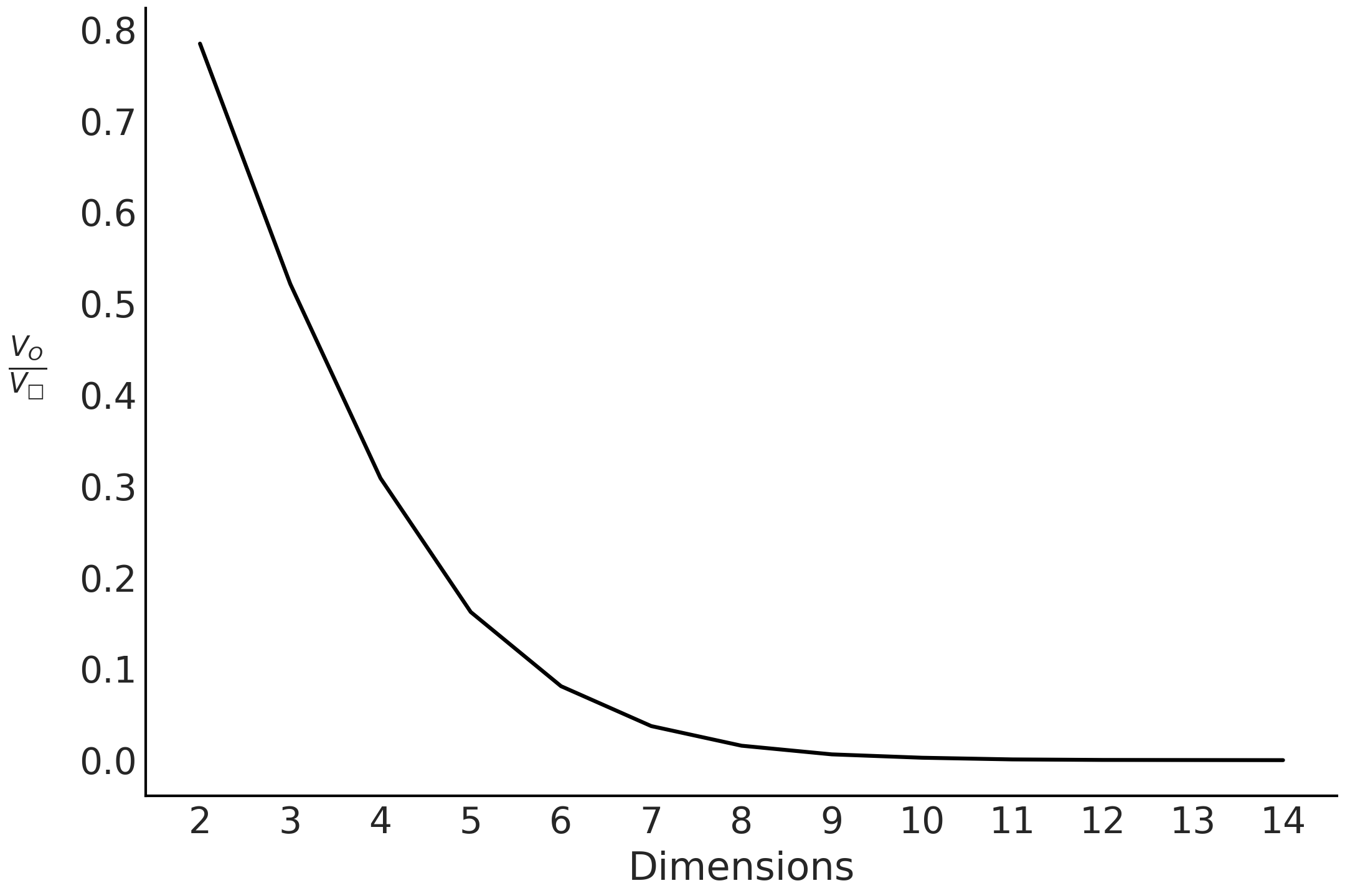
Fig. 11.28 As we increase the dimensions the chance of getting a point inside an hypersphere inscribed into a hyper-cube goes to zero. This shows that in higher dimensions, almost all of the volume of an hypercube is in its corners.#
Let us see another examples using Multivariate Gaussian. Fig. 11.29 shows that as we increase the dimensionality of a Gaussian, most of the mass of that Gaussian is located further and further away from the mode. In fact, most of the mass is around an annulus at radius \(\sqrt{d}\) from the mode, in other words as we increase the dimensionality of the Gaussian the mode becomes less and less typical. In higher dimensions the mode, which is also the mean, is actually an outlier. The reason is that it is very unusual for any given point to be average in all dimensions!
We can also see this from another perspective. The mode is always the point with highest density, even if in high dimensional space. The key insight is noting that it is unique (like the point from flatland!). If we move away from the mode we will find points that are individually less likely but there are a lot of them. As we saw in Section Continuous Random Variables and Distributions a probability is computed as the integral of the density over a volume (actually an interval in the one dimensional case), so to find out where all the mass of a distribution is we have to balance both the density and their volume. As we increase the dimension of the Gaussian we will be most likely to pick a point from an annulus that excludes the mode. The region of the space containing most of the mass of a probability distribution is known as the typical set. In Bayesian statistics we care about it, because if we are going to approximate a high dimensional posterior with samples it suffices that the samples come from the typical set.
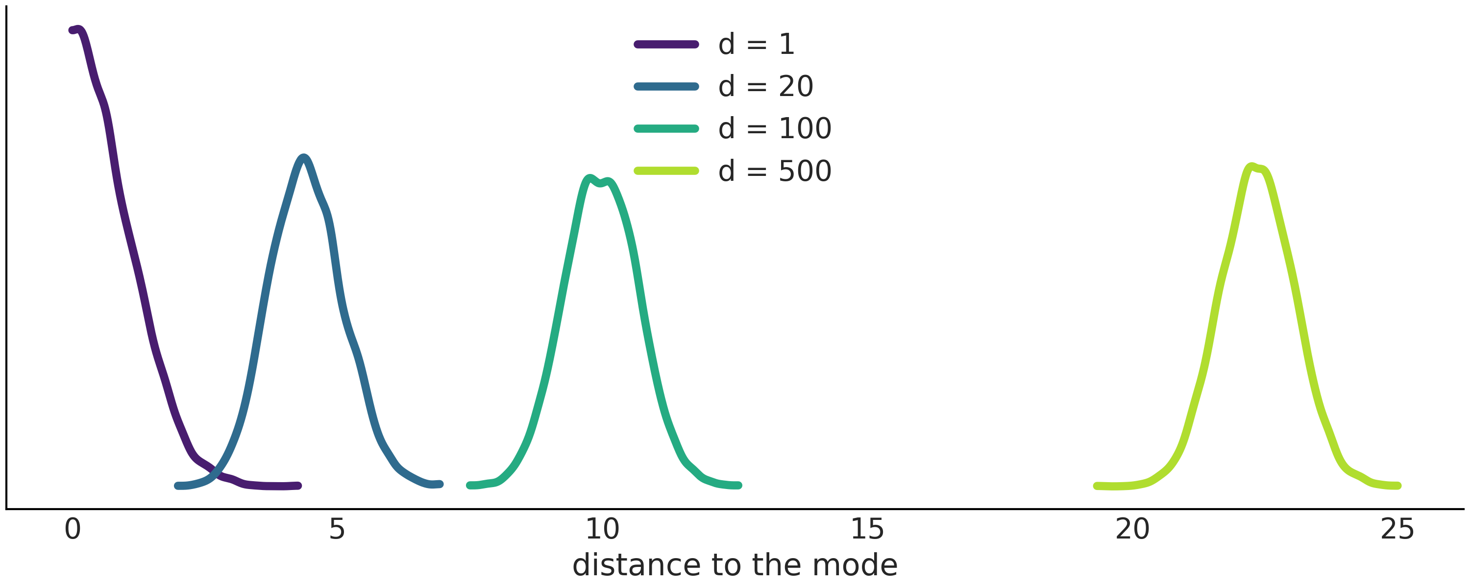
Fig. 11.29 As we increase the dimension of a Gaussian most of the mass is distributed farther and farther away from the mode of that Gaussian.#
11.9. Inference Methods#
There a a myriad of methods to compute the posterior. If we exclude the exact analytical solutions we already discussed in Chapter 1 when we discussed conjugate priors, we can classify inference methods into 3 large groups:
Deterministic integration methods, that we have not yet seen in the book, but we will do next
Simulations methods, also introduced in Chapter 1 and the methods of choice through out the entire book and finally
Approximation methods, for example, the ABC method discussed in Chapter 8, in the case that the likelihood function does not have a closed form expression.
While some methods could be combinations of these categories, we still think it is useful as to order the plethora of available methods.
For a good chronological tour of Bayesian computation methods over the past two and a half centuries, with an special emphasis on those that transformed Bayesian inference we recommend you read Computing Bayes: Bayesian Computation from 1763 to the 21st Century [145]
11.9.1. Grid Method#
The grid method is a simple brute-force approach. We want to know the value of posterior distribution over its domain to be able to use it (finding the maximum, computing expectation, etc). Even if you are not able to compute the whole posterior, you may be able to evaluate the prior and the likelihood density function point-wise; this is a pretty common scenario, if not the most common one. For a single parameter model, the grid approximation is:
Find a reasonable interval for the parameter (the prior should give some hints).
Define a grid of points (generally equidistant) on that interval.
For each point in the grid, multiply the likelihood and the prior. Optionally, we may normalize the computed values so the posterior sum to 1 by dividing the result at each point by the sum of all points
Code Block grid_method computes the posterior the Beta-Binomial model:
def posterior_grid(ngrid=10, α=1, β=1, heads=6, trials=9):
    grid = np.linspace(0, 1, ngrid)
    prior = stats.beta(α, β).pdf(grid)
    likelihood = stats.binom.pmf(heads, trials, grid)
    posterior = likelihood * prior
    posterior /= posterior.sum()
    return posterior
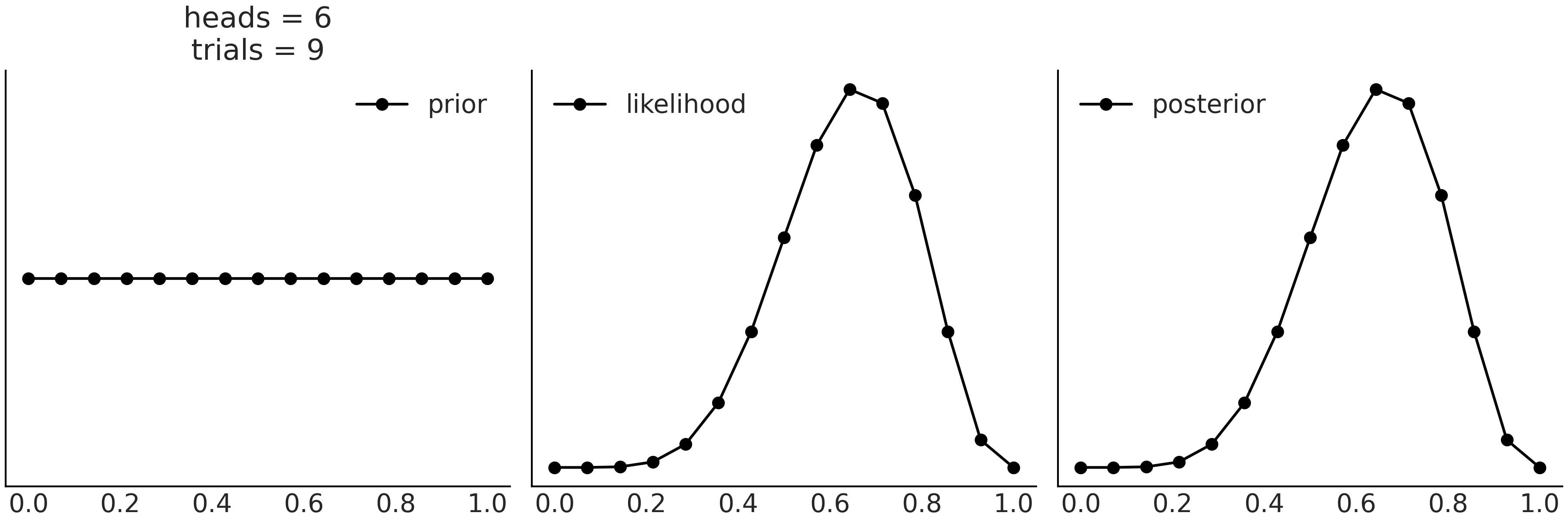
Fig. 11.30 By evaluating the prior and the likelihood pointwise over a grid we can approximate the posterior.#
We can get a better approximation by increasing the number of points of the grid. In fact if we use infinite number of points we will get the exact posterior, at the cost of needing infinite computing resources. The biggest caveat of the grid approach is that this method scales poorly with the number of parameters as explained in Moving out of Flatland.
11.9.2. Metropolis-Hastings#
We introduced Metropolis-Hastings algorithm [7, 8, 9] very early in Section A DIY Sampler, Do Not Try This at Home and show a simple Python implementation in Code Block metropolis_hastings. We will now provide more detail about why this method works. We will do it using the language of Markov Chains introduced in Section Markov Chains.
The Metropolis-Hastings algorithm is a general method that allow us to start with any irreducible Markov chain on the state space of interest and then modify it into a new Markov chain that has the stationary distribution that we really care. In other words we take samples from an easy to sample distribution like a Multivariate Normal and we turn those samples into samples from our target distribution. The way we modify the original chain is by being selective, we only accept some of the samples and reject the others. As we saw in Chapter 1. The probability of accepting a new proposal is:
Let us rewrite this in a shorter form, for easier manipulation.
That is we propose with probability \(q_{ij}\) (read the subscript \(ij\) as from \(i\) to \(j\)) and accepts the proposal with probability \(a_{ij}\). One of the nice feature of this method is that we do not need to know the normalizing constant of the distribution we want to sample, as it will be cancelled out when we compute \(\frac{p_j}{p_i}\). This is very important because in may many problems, including Bayesian inference, computing that normalization constant (the marginal likelihood) is very difficult.
We will now show that the Metropolis-Hastings chain is reversible with stationary distribution \(p\) as we mentioned in Section Markov Chains. We need to proof that the detailed balance condition i.e. the reversibility condition holds, that is:
Let \(\mathbf{T}\) be the transition matrix, we just need to show that \(p_i t_{ij} = p_j t_{ji}\) for all \(i\) and \(j\), this is trivial when \(i = j\) so we assume that \(i \neq j\), we can write:
Meaning that the probability to transition from \(i\) to \(j\) is the probability of proposing the move times the probability of accepting it. Let us first see the case where the probability of acceptance is less that 1, this happens when \(p_j q_{ji} \le p_i q_{ij}\), then we have that
and also
Using Equation (11.89), we have
replacing \(a_{ij}\) in Equation (11.90)
simplifying above we get:
Because \(a_{ji} = 1\) we can include it without changing the validity of the equation.
which finally we get that
By symmetry when \(p_j q_{ji} > p_i q_{ij}\) we will arrive at the same result. As the reversibility condition holds, \(p\) is the stationary distribution of our Markov chain with transition matrix \(\mathbf{T}\).
The above proof gives us the theoretical confidence that we can use Metropolis-Hastings to sample from virtually any distribution we want. We can also see that while this is a very general result, it does not help us to choose a proposal distribution. In practice the proposal distribution is very important as the efficiency of the method depends heavily on this choice. In general it is observed that if the proposal makes large jumps the probability of acceptance is very low, and the method spend most of the time rejecting new states and thus stuck in one place. On the contrary if the proposal takes too small jumps the acceptance rate is high but the exploration is poor, as the new states are in a small neighborhood of the old state. A good proposal distribution is one that generates new putative states far away from the old state with high acceptance rate. This is generally difficult to do if we do not know the geometry of the posterior distribution, but that is precisely what we want to find out. In practice useful Metropolis-Hastings methods are those that are adaptive [146, 147, 148, 149]. For example, we can use a Multivariate Gaussian distribution as proposal distribution. During tuning we can compute the empirical covariance from the posterior samples and use it as the covariance matrix of the proposal distribution. We can also scale the covariance matrix so that the average acceptance rate approach a predefined acceptance rate [150, 151, 152]. In fact there is evidence that under certain circumstances and when the dimensionality of the posterior increases the optimal acceptance rate converges to the magic number 0.234 [150]. In practice it seems that an acceptance rate around 0.234 or a little bit higher gives more or less the same performance but the general validity and useful of this result has also been disputed [153, 154].
In the next section we will discuss a clever way to generate proposals that help to correct most of the problems with basic Metropolis-Hastings.
11.9.3. Hamiltonian Monte Carlo#
Hamiltonian Monte Carlo (HMC) [25] [155, 156, 157] is a type of MCMC method that makes use of gradients to generate new proposed states. The gradients of the log-probability of the posterior evaluated at some state provides information of the geometry of the posterior density function. HMC attempts to avoid the random walk behavior typical of Metropolis-Hastings by using the gradient to propose new positions far from the current one with high acceptance probability. This allows HMC to better scale to higher dimensions and in principle more complex geometries, than alternatives.
In simple terms, a Hamiltonian is a description of the total energy of a physical system. We can decompose the total energy into two terms, the kinetic and the potential energy. For a real system like rolling a ball down a hill, the potential energy is given by the position of the ball. The higher the ball the higher the potential energy. The kinetic energy is given by the velocity of the ball, or more correctly by its momentum (which takes into account both the velocity and the mass of the object). We will assume the total energy preserves, meaning that if the system gains kinetic energy then is because it has lost the same amount of potential energy. We can write the Hamiltonian of such a systems as:
where \(K(\mathbf{p}, \mathbf{q})\) is called the kinetic energy, and \(V(\mathbf{q})\) is the potential energy. The probability of finding the ball at a particular position with a particular momentum is then given by:
To simulate such a systems we need to solve the so called Hamiltonian equations:
Note that \(\frac{\partial V}{\partial \mathbf{p}} = \mathbf{0}\).
Because we are not interested in modeling an idealized ball rolling down an idealized hill, but to model an idealized particle along the posterior distribution, we need to make a few adjustments. First the potential energy is given by the probability density we are trying to sample from \(p(\mathbf{q})\). For the momentum we are just going to invoke an auxiliary variable. That is, a made up variable that will help us. If we choose \(p(\mathbf{p} \mid \mathbf{q})\) then we can write:
This ensures us that we can recover our target distribution by marginalize out the momentum. By introducing the auxiliary variable, we can keep working with the physical analogy, and later remove the auxiliary variable and go back to our problem, sampling the posterior. If we replace Equation (11.100) in Equation (11.98) we got:
As explained previously, the potential energy \(V(\mathbf{q})\) is given by the \(p(\mathbf{q})\) the density function of the target posterior distribution, and we are free to choose the kinetic energy. If we choose it to be Gaussian, and drop the normalization constant, we have:
where \(M\) is the precision matrix that parameterized the Gaussian distribution (also referred to as the mass matrix in Hamiltonian Monte Carlo literature). And if we choose \(M = I\), i.e. the identity matrix which is \(n \times n\) square matrix with ones on the main diagonal and zeros elsewhere, we have:
This makes calculations easier as now
and
We can then simplify Hamilton’s equations to:
Summarizing,the HMC algorithm is then:
Sample a \(\mathbf{p} \sim \mathcal{N}(0, I)\)
Simulate \(\mathbf{q}_t\) and \(\mathbf{p}_t\) for some amount of time \(T\)
\(\mathbf{q}_T\) is our new proposed state
Use the Metropolis acceptance criterion to accept or reject \(\mathbf{q}_T\).
Why we still need to use the Metropolis acceptance criterion? Intuitively because we can think of HMC as a Metropolis-Hasting algorithm with a better proposal distribution. But there is also a very good numerical justification, because this steps corrects for errors introduced by the numerical simulation of the Hamiltonian equations.
To compute the Hamiltonian equations we have to compute a trajectory of the particle, i.e. all the intermediate points between one state and the next. In practice this involves computing a series of small integration steps using an integrator method. The most popular one is the leapfrog integrator. Leapfrog integration is equivalent to updating positions \(q_t\) momentum \(q_t\) at interleaved time points, staggered in such a way that they leapfrog over each other.
Code Block leapfrog shows a leapfrog
integrator implemented in Python [26]. The arguments are: q and p
the initial position and momentum respectively. dVdq is a Python
function that returns the gradient of the position of some target
density function at position q
\(\frac{\partial V}{\partial \mathbf{q}}\). We used JAX [116]
auto-differentiation ability to generate this function. path_len
indicates how long to integrate for and step_size how large each
integration step should be. As a result we obtain a new position and
momentum as output of the function leapfrog.
def leapfrog(q, p, dVdq, path_len, step_size):
    p -= step_size * dVdq(q) / 2  # half step
    for _ in range(int(path_len / step_size) - 1):
        q += step_size * p  # whole step
        p -= step_size * dVdq(q)  # whole step
    q += step_size * p  # whole step
    p -= step_size * dVdq(q) / 2  # half step

    return q, -p  # momentum flip at end
Note that in function leapfrog we flip the sign of the output
momentum. This is the simplest way to achieve a reversible
Metropolis-Hastings proposal, as it augment the numerical integration
with a negative step.
We have now all the ingredients to implement a HMC method in Python, as
in Code Block hamiltonian_mc. Like our previous
Metropolis-Hasting example in Code Block metropolis_hastings this is
not meant to be use for serious model inference but instead a simple
example to demonstrate the method. The arguments are n_samples the
number of samples to return, negative_log_prob the negative log
probability to sample from, initial_position the initial position to
start sampling, path_len, step_size, as a result we obtain sample
from the target distribution.
def hamiltonian_monte_carlo(
    n_samples, negative_log_prob, initial_position,
    path_len, step_size):
    # autograd magic
    dVdq = jax.grad(negative_log_prob)

    # collect all our samples in a list
    samples = [initial_position]

    # Keep a single object for momentum resampling
    momentum = stats.norm(0, 1)
    # If initial_position is a 10d vector and n_samples is 100, we want
    # 100 x 10 momentum draws. We can do this in one call to momentum.rvs, and
    # iterate over rows
    size = (n_samples,) + initial_position.shape[:1]
    for p0 in momentum.rvs(size=size):
        # Integrate over our path to get a new position and momentum
        q_new, p_new = leapfrog(
            samples[-1], p0, dVdq, path_len=path_len, step_size=step_size,
        )

        # Check Metropolis acceptance criterion
        start_log_p = negative_log_prob(samples[-1]) - np.sum(momentum.logpdf(p0))
        new_log_p = negative_log_prob(q_new) - np.sum(momentum.logpdf(p_new))
        if np.log(np.random.rand()) < start_log_p - new_log_p:
            samples.append(q_new)
        else:
            samples.append(np.copy(samples[-1]))

    return np.array(samples[1:])
Fig. 11.31 shows 3 different trajectories around the same 2D normal distribution. For practical sampling we do not want the trajectories to be circular, because they will arrive at the same position that we started at. Instead we want to move as far as possible from our starting point, for example, by avoiding U-turns in the trajectory, and hence the name of one of the most popular dynamic HMC method No U-Turn Sampling (NUTS).
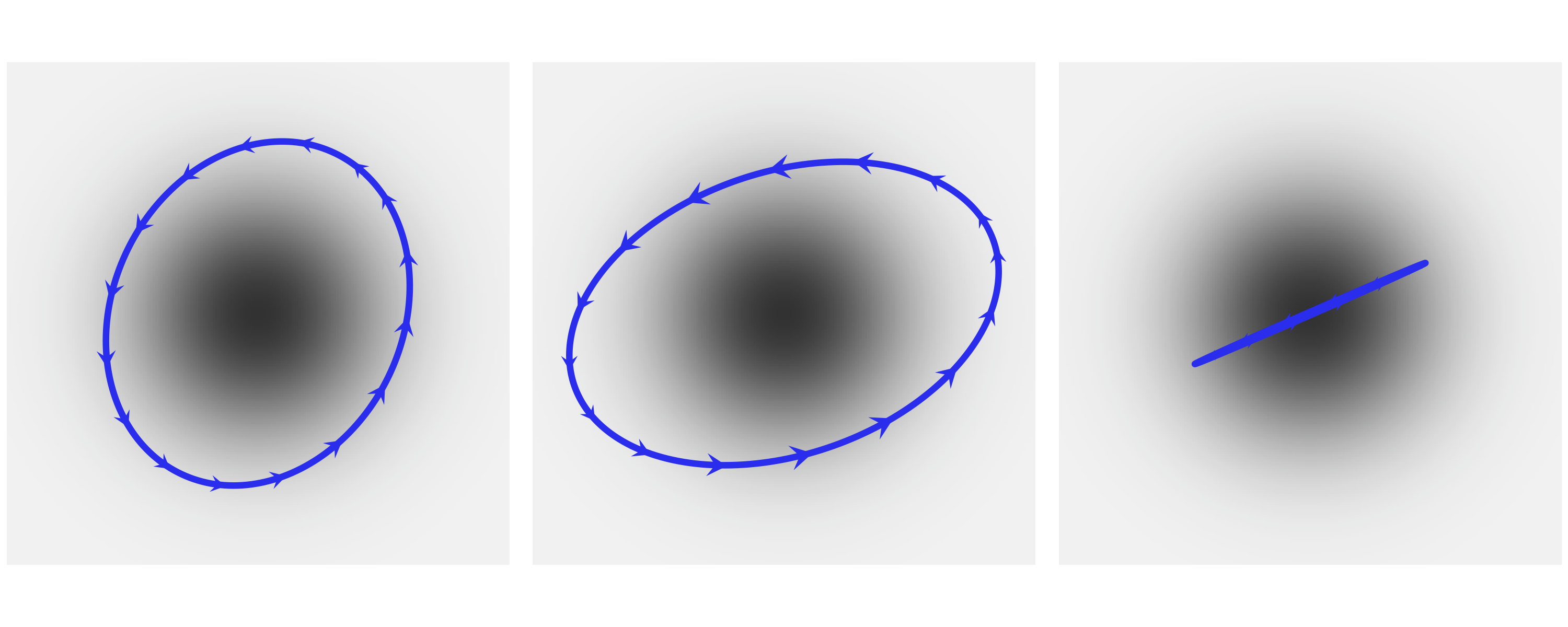
Fig. 11.31 Three HMC trajectories around a 2D multivariate normal. The momentum is indicated by the size and direction of the arrows, with small arrows indicating small kinetic energy. All these trajectories are computed in such a way that they end at their starting position, which completing an elliptical trajectory.#
We show another example in Fig. 11.32, which contains 3 different trajectory around the same Neal’s funnel, a common geometry arising in (centered) hierarchical models as we showed in Section Posterior Geometry Matters. This is an example of a trajectory failing to properly simulate following the correct distribution, we call such trajectories divergent trajectories, or simply divergences. They are useful diagnostics as explained in Section Divergences. Usually, Symplectic integrators like leapfrog integrator are highly accurate even for long trajectories, as they tend to be tolerant of small errors and oscillate around the correct trajectory. Moreover, these small errors can be corrected exactly by applying the metropolis criteria to accept or reject the Hamiltonian proposal. However, there is an importance exception to this ability to generate small, easy to fix errors: when the exact trajectories lie on regions of high curvature, the numerical trajectories generated by symplectic integrators can diverge, generating trajectory that rapidly get off towards the boundaries of the distribution we are trying to explore.
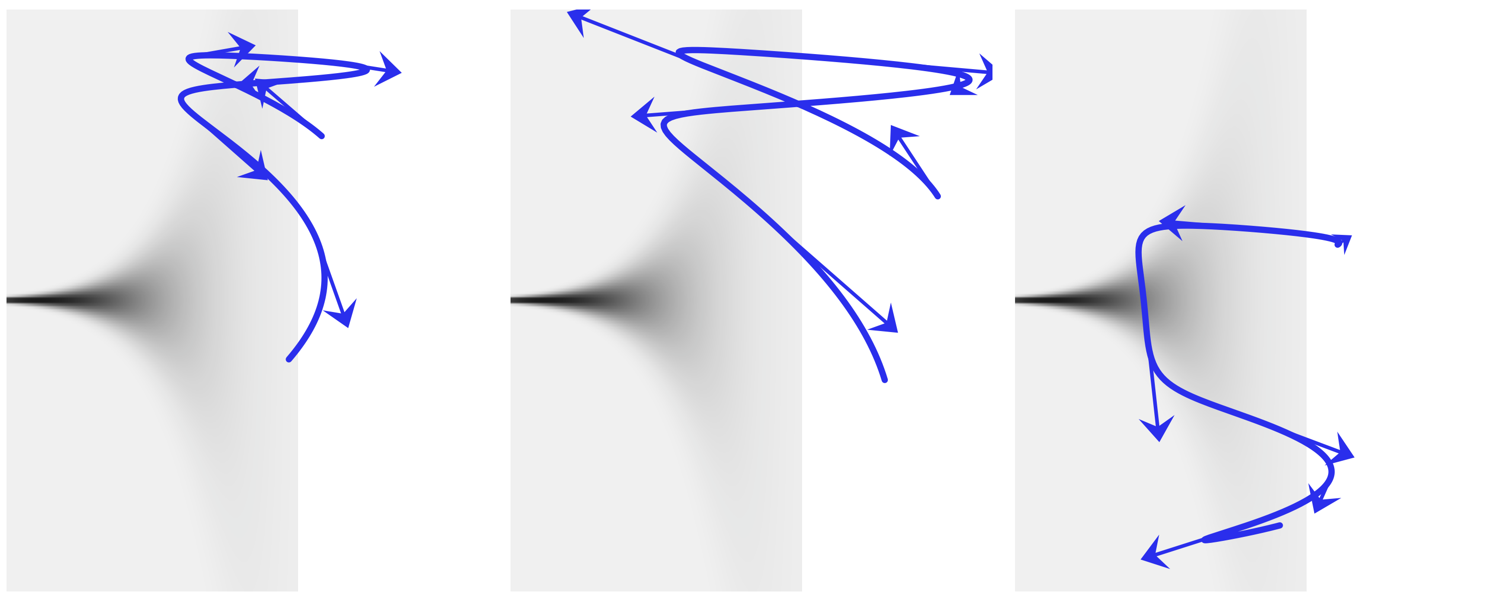
Fig. 11.32 Three HMC trajectories around a 2D Neal’s funnel. This kind geometry turns up in centered hierarchical models. We can see that all these trajectories went wrong. We call this kind of trajectories divergences and can be used as a diagnostic of HMC samplers.#
Both Figures Fig. 11.31 and Fig. 11.32 highlight the fact that an efficient HMC method requires proper tuning of its hyperparameters. HMC has three hyparameters:
the time discretization (step size of the leapfrog)
the integration time (number of leapfrog steps)
the precision matrix \(M\) that parameterized the kinetic energy
For example, if the step size is too large, the leapfrog integrator will be inaccurate and too many proposals will be rejected. However, if it is too small we will waste computation resources. If the number of steps is too small, the simulated trajectory at each iteration will be too short and sampling will fall back to random walk. But if it is too large the trajectory might runs in circles and we again waste computation resources. If the estimated covariance (inverse of the precision matrix) is too different from the posterior covariance, the proposal momentum will be suboptimal and the movement in the position space will be too large or too small in some dimension.
Adaptive dynamics Hamiltonian Monte Carlo methods, like those used by
default in PyMC3, Stan and other PPLs can adapt these hyperparameters
automatically during the warm-up or tuning phase. The step size can be
learning automatically by adjusting it to match a predefined
acceptance-rate target. For example, in PyMC3 you set the argument
target_accept [27] The precision matrix \(M\) or its inverse can be
estimated from the samples during warm-up phase and the number of steps
can be dynamically adapted at each MCMC step using the NUTS algorithm
[158]. In order to avoid too long trajectory that could go near
the initialization point, NUTS extends the trajectory backward and
forwards until a U-turn criterion is met. Additionally, NUTS applies a
multinomial sampling to choose from all the generated points from the
trajectory, as this provides a better criteria for efficient exploration
of the target distribution (sampling from the trajectory could be done
with fixed integration time HMC as well).
11.9.4. Sequential Monte Carlo#
Sequential Monte Carlo is a family of Monte Carlo methods also known as particle filters. It has wide application to Bayesian inference for static models and dynamic models such as sequential time series inference and signal processing [63, 159, 160, 161]. There are many variations and implementation under the same or similar name, with different application. Thus you might at times find the literature a bit confusing. We will give a brief description of the SMC/SMC-ABC method as implemented in PyMC3 and TFP. For a detailed discussion of SMC methods under a unified framework we recommend the book An Introduction to Sequential Monte Carlo [63].
First note that we can write the posterior in the following way:
When \(\beta = 0\) we see that \(p(\boldsymbol{\theta} \mid Y)_{\beta}\) is the prior and when \(\beta = 1\) we see that \(p(\boldsymbol{\theta} \mid Y)_{\beta}\) is the true posterior [28].
SMC proceeds by increasing the value of \(\beta\) in \(s\) successive stages \(\{\beta_0=0 < \beta_1 < ... < \beta_s=1\}\). Why is this a good idea? There are two related ways to justify it. First, the stepping stones analogy. Instead of directly trying to sample from the posterior we begin by sampling from the prior, which is generally easier to do. Then we add some intermediate distributions until we reach the posterior (see Fig. 8.2). Second is the temperature analogy. The \(\beta\) parameters is analogue to the inverse temperature of a physical system, as we decrease its value (increase the temperature) the system is able to access to more states, and as we decrease its value (decrease the temperature) the system “freezes” into the posterior [29]. Fig. 8.2 shows an hypothetical sequence of tempered posteriors. The use of the temperature (or its inverse) as an auxiliary parameter is known as tempering, the term annealing is also common [30].
The SMC method, as implemented in PyMC3 and TFP, can be summarized as follows:
Initialize \(\beta\) at zero.
Generate \(N\) samples \(s_{\beta}\) from the tempered posterior.
Increase \(\beta\) in order to keep the effective sample size [31] at a predefined value.
Compute a set of \(N\) importance weights \(W\). The weights are computed according to the new and old tempered posterior.
Obtain \(s_w\) by resampling \(s_{\beta}\) according to \(W\).
Run \(N\) MCMC chains for \(k\) steps, starting each one from a different sample in \(s_w\) and retaining only the samples in the last step.
Repeat from step 3 until \(\beta=1\)
The resampling step works by removing samples with a low probability and replacing them with samples with a higher probability. This step decreases the diversity of the samples. Then, the MCMC step perturbs the samples, hopefully increasing the diversity and therefore helping SMC to explore the parameter space. Any valid MCMC transition kernel could be used in SMC, and depending on your problem you might find some perform better than others. For example, with ABC methods we generally need to rely on gradient-free methods such as Random Walk Metropolis-Hasting as the simulators are generally not differentiable.
The efficiency of the tempered method depends heavily on the intermediate values of \(\beta\). The smaller the difference between two successive values of \(\beta\), the closer the two successive tempered posteriors will be, and thus the easier the transition from one stage to the next. But if the steps are too small, we will need many intermediate stages, and beyond some point this will waste a lot of computational resources without really improving the accuracy of the results. Another important factor is the efficiency of the MCMC transitional kernel that adds diversity to the samples. To help improve the efficiency of the transition, PyMC3 and TFP uses the samples from the previous stage to tune the proposal distribution of the current stage and also the number of steps taken by the MCMC, with the number of steps being the same across all chains.
11.9.5. Variational Inference#
While we do not use variational inference in this book, it is a useful approach to know about. Compared to MCMC, VI tends to be easier to scale to large data and is faster to run computationally, but with less theoretical guarantees of convergence [162].
As we previously mentioned in Section Kullback-Leibler Divergence, we can use one distribution to approximate another and then use the Kullback-Leibler (KL) divergence to measure how good the approximation is. Turns out we can use this approach to do Bayesian inference as well! Such approach is called variational inference (VI) [163]. The goal of VI is to approximate the target probability density, in our case the posterior distribution \(p(\boldsymbol{\theta} \mid Y)\), with a surrogate distribution \(q(\boldsymbol{\theta})\). In practice we usually choose \(q(\boldsymbol{\theta})\) to be of simpler form than \(p(\boldsymbol{\theta} \mid Y)\), and we find the member of that family of distributions, which is the closest to the target in the KL divergence sense, using optimization. With small rewrite to Equation (11.41), we have:
However, this objective is hard to compute because it requires the marginal likelihood of \(p(Y)\). To see that let us expand Equation (11.108):
Luckily, since \(\log{p(Y)}\) is a constant with respect to \(q(\boldsymbol{\theta})\), we can omit it during optimization. Thus, in practice, we maximize the evidence lower bound (ELBO) as shown in Equation (11.110), which is equivalent to minimizing the KL divergence:
The last piece of the puzzle is to figure out how to compute the expectation in Equation (11.110). Instead of solving an expensive integration, we compute the average using Monte Carlo samples drawn from the surrogate distribution \(q(\boldsymbol{\theta})\) and plug them into (11.110).
The performance of VI depends on many factors. One of them being the family of surrogate distributions we choose from. For example, a more expressive surrogate distribution helps capture more complex, nonlinear dependencies among components of the target posterior distribution, and thus usually gives better result (see Fig. 11.33). Automatically choosing a good surrogate family distribution and efficiently optimizing it is currently an active research area. Code Block vi_in_tfp shows a simple example of using VI in TFP, with two different types of surrogate posterior distributions. The result is shown in Fig. 11.33.
tfpe = tfp.experimental
# An arbitrary density function as target
target_logprob = lambda x, y: -(1.-x)**2 - 1.5*(y - x**2)**2

# Set up two different surrogate posterior distribution
event_shape = [(), ()]  # theta is 2 scalar
mean_field_surrogate_posterior = tfpe.vi.build_affine_surrogate_posterior(
    event_shape=event_shape, operators="diag")
full_rank_surrogate_posterior = tfpe.vi.build_affine_surrogate_posterior(
    event_shape=event_shape, operators="tril")

# Optimization
losses = []
posterior_samples = []
for approx in [mean_field_surrogate_posterior, full_rank_surrogate_posterior]:
    loss = tfp.vi.fit_surrogate_posterior(
        target_logprob, approx, num_steps=100, optimizer=tf.optimizers.Adam(0.1),
        sample_size=5)
    losses.append(loss)
    # approx is a tfp distribution, we can sample from it after training
    posterior_samples.append(approx.sample(10000))
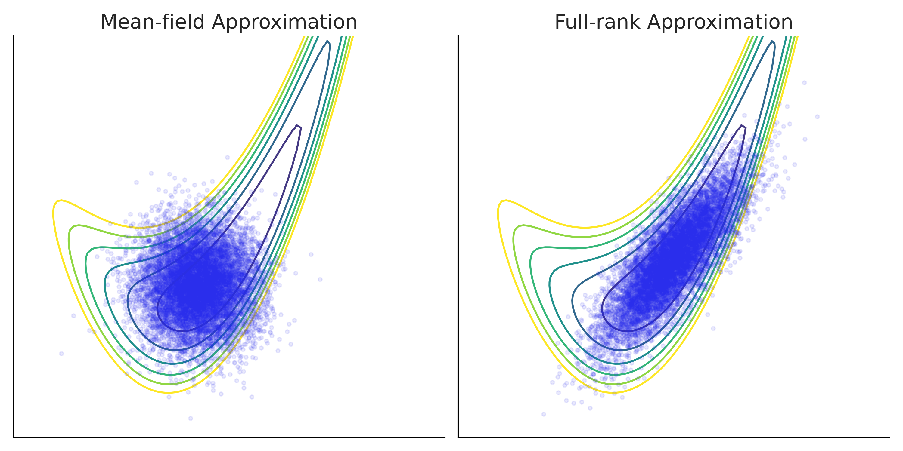
Fig. 11.33 Using variational inference to approximate a target density function. The target density is a 2D banana shaped function plotted using contour lines. Two types of surrogate posterior distributions are used for the approximation: on the left panel a mean-field Gaussian (one univariate Gaussian for each dimension with trainable location and scale) and on the right panel a full-rank Gaussian (a 2D multivariate Gaussian with trainable mean and covariance matrix) [164]. Samples from the approximation after optimization are plotted as dots overlay on top of the true density. Comparing the two, you can see that while both approximations does not fully capture the shape of the target density, full-rank Gaussian is a better approximation thanks to its more complex structure.#
11.10. Programming References#
Part of computational Bayes is well, the computer and the software tools now available. Using these tools help modern Bayesian practitioner share models, reduce mistakes, and speed up the model building and inference process. To have the computer work for us we need to program it but often this is easier said than done. To use them effectively still requires thought and understanding. In this last section we will provide some high level guidance for the major concepts.
11.10.1. Which Programming Language?#
There are many programming languages. We primarily used Python, but other popular languages such as Julia, R, C/C++ exist with specialized application for Bayesian computation as well. So which programming language should you use? There is no universal right or wrong answer here. Instead you should always consider the complete ecosystem. In this book we use Python because packages like ArviZ, Matplotlib, and Pandas to make data processing and displaying easy. This is not exclusive to Python. For a Bayesian specifically consider the PPLs available in that particular language, because if none exists then you might want to reconsider your programming language of choice. Also consider the community you want to work with and what language they use. One of the authors of this book lives in Southern California, so knowing English, and a bit of Spanish makes a lot of sense, because with those two he could communicate in common situations. It is the same with programming languages, if your future lab group uses R then learning R is a good idea.
Computational purists may exclaim that some languages are faster than others computationally. This of course is true but we advise not getting too wrapped up in the discussion of “which is the fastest ppl”. In real life scenarios different models take different amount of time to run. Additionally there is “human time” which is the time for one to iterate and come up with a model, and “model run time” which is the time it takes for the computer to return a useful result. These are not the same and in different situations one is more important than the other. This is all to say, do not worry too much about picking the “right” up front language, if you learn one effectively the concepts will transfer to another.
11.10.2. Version Control#
Version control is not necessary but is absolutely recommended and will incur great benefits if utilized. When working alone, version control lets you iterate through model designs without worry about losing your code or making changes or experiment that breaks your model. This by itself lets you iterate quicker and with more confidence, as well as the ability to switch back and forth between different model definitions. When working with others, version control enables collaboration and code sharing, that would be challenging or impossible to perform without the snapshotting or comparison features that version control systems allows. There are many different version control systems (Mercurial, SVN, Perforce) but git is currently the most popular. Version control is not typically tied to a particular programming language.
11.10.3. Dependency Management and Package Repositories#
Nearly all code relies on other code to run (it is turtles all the way down). PPLs in particular rely on a lot of different libraries to run. We strongly suggest familiarizing yourself with a requirements management tool that helps you see, list, and freeze the packages your analysis relies on. Additionally package repositories are where these requirement packages are fetched from. These are typically specific to the language, for example, one requirements management tool in Python is pip, and a popular cloud repository is pypi. In Scala sbt is one tool that helps with dependencies and Maven is a popular package repository. All mature languages will have this tooling, but you must make the conscious choice to use them.
11.10.4. Environment Management#
All code executes in an environment. Most people forget this until their code suddenly stops working, or does not work on another computer. Environment management is the set of tools used to create a reproducible computation environment. This is of particular importance to Bayesian Modelers who deal with enough randomness in their models, and do not want the computer to add an additional layer of variability. Unfortunately Environment Management is also one of the most confusing portions of programming. In general there are two rough types of environment control, language specific and language agnostic. In Python virtualenv is a python specific environment manager, whereas containerization and virtualization are language agnostic. We have no specific suggestion here as the choice depends largely on your comfort with these tool, and also where you plan to run the code. We do absolutely recommend making a deliberate choice here though, as it makes sure you have reproducible results.
11.10.5. Text Editor vs Integrated Development Environment vs Notebook#
When writing code, you must well, write it somewhere. For data minded folks there are typically three interfaces for this.
The first and simplest is a text editor. The most basic text editors allow you to, surprise, edit text and save it. With these editors you can write a python program, save it, and then run it. Typically text editors are very “light weight” and do not include much extra functionality besides basic things like find and replace. Think of text editors like a bicycle. They are simple, their interface is basically a handlebar and some pedals, and they will get you from here to there but its mostly on you to do the work.
Integrated Development Environments (IDE) by comparison the modern airplanes. They have an insane amount of functionality, a lot buttons, and a lot of automation. IDEs let you edit text at their core, but as the name suggests they integrate many other aspects of development as well. For example, functionality for running code, unit-testing, linting code, version control, code version comparison, and much much more. IDEs are typically most useful when writing a lot of complicated code that spans many modules.
While we would love to provide a simple definition of a text editor vs IDE, the line these days is very blurry. Our suggestion is start more on the text editor side and move to IDEs once familiar with how code works. Otherwise it will be hard for you to tell what the IDE is doing for you “under the hood”.
Notebooks are an entirely different interface. Notebooks are special in they mix code, output, and documentation, as well as allowing nonlinear code execution. For this book the majority of the code, and figures, are presented in Jupyter Notebook files. We also provide links to Google Colab which a cloud notebook environment. Notebooks are typically best used for exploratory data analysis, and explanatory type situations, such as this book. They are not so well suited for running production code.
Our suggestion for notebooks is similar to IDEs. If new to statistical computing start with a text editor first. Once you have a strong handle of how to run code from individual files, then move to notebook environments, either a cloud hosted Google colab, or Binder instance, or a local Jupyter Notebook
11.10.6. The Specific Tools Used for this Book#
Here is what we used for this book. This does not mean these are the only tools you can use, these are just the ones we used.
Programming Language: Python
Probabilistic Programming Languages: PyMC3, TensorFlow Probability. Stan and Numpyro are displayed briefly as well.
Version control: git
Dependency Management: pip and conda
Package repository: pypi, conda-forge
Environment Management: conda
General Documentation: LaTeX (for book writing), Markdown (for code package), Jupyter Notebooks