Code 4: Extending Linear Models

This is a reference notebook for the book Bayesian Modeling and Computation in Python

The textbook is not needed to use or run this code, though the context and explanation is missing from this notebook.

If you’d like a copy it’s available from the CRC Press or from Amazon. ``

import pymc3 as pm
import matplotlib.pyplot as plt
import arviz as az
import pandas as pd
import numpy as np
from scipy import stats

import theano.tensor as tt
import theano

import datetime
print(f"Last Run {datetime.datetime.now()}")

Last Run 2021-11-19 16:44:33.955392

az.style.use("arviz-grayscale")
plt.rcParams['figure.dpi'] = 300 

Transforming Covariates

Code 4.1

babies = pd.read_csv('../data/babies.csv')

# Add a constant term so we can use a the dot product approach
babies["Intercept"] = 1

babies.head()

	Month	Length	Intercept
0	0	48.5	1
1	0	50.5	1
2	0	50.5	1
3	0	52.0	1
4	0	47.5	1

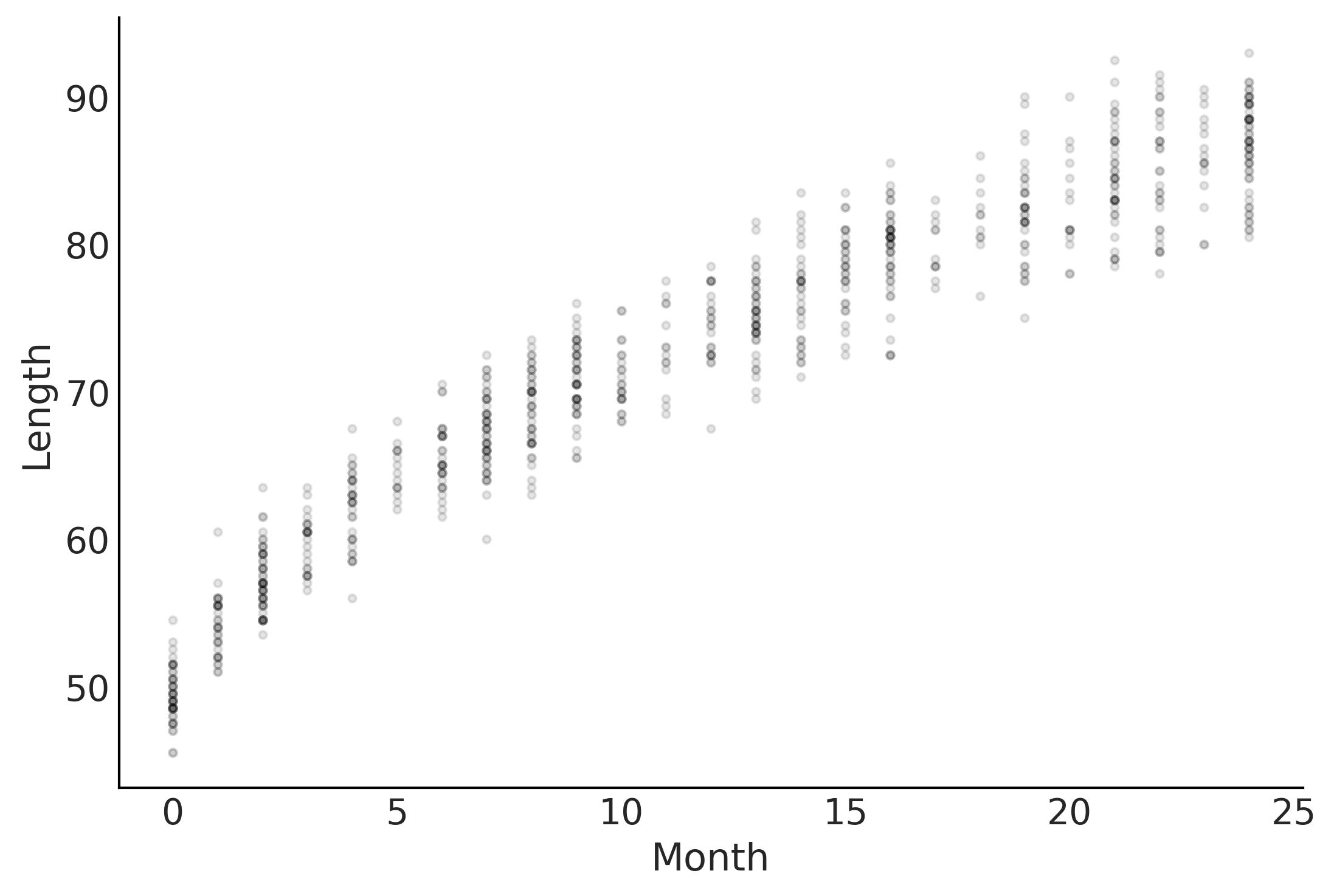
Figure 4.1

fig, ax = plt.subplots()

ax.plot(babies["Month"], babies["Length"], 'C0.', alpha=0.1)
ax.set_ylabel("Length")
ax.set_xlabel("Month");
plt.savefig('img/chp04/baby_length_scatter.png', dpi=300)

Code 4.2

with pm.Model() as model_baby_linear:
    β = pm.Normal('β', sigma=10, shape=2)
    
    # Use dot product instead of expanded multiplication
    μ = pm.Deterministic("μ", pm.math.dot(babies[["Intercept", "Month"]], β))
    ϵ = pm.HalfNormal("ϵ", sigma=10)

    length = pm.Normal("length", mu=μ, sigma=ϵ, observed=babies["Length"])

    trace_linear = pm.sample(draws=2000, tune=4000)
    pcc_linear = pm.sample_posterior_predictive(trace_linear)
    inf_data_linear = az.from_pymc3(trace=trace_linear,
                                    posterior_predictive=pcc_linear)

/var/folders/7p/srk5qjp563l5f9mrjtp44bh800jqsw/T/ipykernel_8872/2954483905.py:10: FutureWarning: In v4.0, pm.sample will return an `arviz.InferenceData` object instead of a `MultiTrace` by default. You can pass return_inferencedata=True or return_inferencedata=False to be safe and silence this warning.
  trace_linear = pm.sample(draws=2000, tune=4000)
Auto-assigning NUTS sampler...
Initializing NUTS using jitter+adapt_diag...
Multiprocess sampling (4 chains in 4 jobs)
NUTS: [ϵ, β]

100.00% [24000/24000 00:08<00:00 Sampling 4 chains, 0 divergences]

Sampling 4 chains for 4_000 tune and 2_000 draw iterations (16_000 + 8_000 draws total) took 18 seconds.
The acceptance probability does not match the target. It is 0.5738214538580835, but should be close to 0.8. Try to increase the number of tuning steps.
The acceptance probability does not match the target. It is 0.8837497551468421, but should be close to 0.8. Try to increase the number of tuning steps.

100.00% [8000/8000 00:06<00:00]

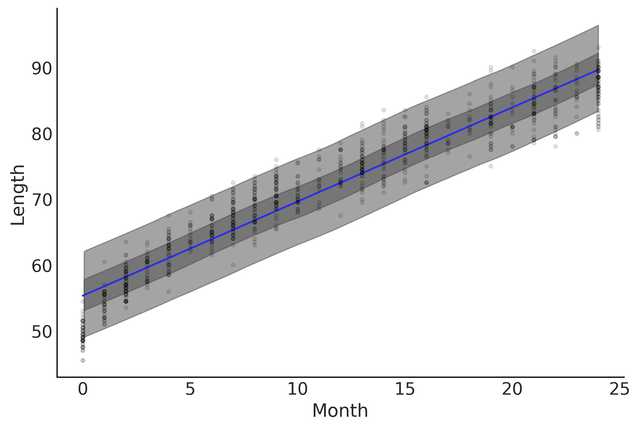
Figure 4.2

fig, ax = plt.subplots()

ax.set_ylabel("Length")
ax.set_xlabel("Month");

μ_m = inf_data_linear.posterior["μ"].values.reshape(-1, babies["Length"].shape[0]).mean(axis=0)

ax.plot(babies["Month"], μ_m, c='C4')
az.plot_hdi(babies["Month"], inf_data_linear.posterior_predictive["length"], hdi_prob=.50, ax=ax)
az.plot_hdi(babies["Month"], inf_data_linear.posterior_predictive["length"], hdi_prob=.94, ax=ax)

ax.plot(babies["Month"], babies["Length"], 'C0.', alpha=0.1)

plt.savefig('img/chp04/baby_length_linear_fit.png', dpi=300)

az.loo(inf_data_linear)

Computed from 8000 by 800 log-likelihood matrix

         Estimate       SE
elpd_loo -2133.32    18.59
p_loo        3.23        -

Code 4.3

with pm.Model() as model_baby_sqrt:
    β = pm.Normal("β", sigma=10, shape=2)

    μ = pm.Deterministic("μ", β[0] + β[1] * np.sqrt(babies["Month"]))
    σ = pm.HalfNormal("σ", sigma=10)

    length = pm.Normal("length", mu=μ, sigma=σ, observed=babies["Length"])
    inf_data_sqrt = pm.sample(draws=2000, tune=4000)

    ppc_baby_sqrt = pm.sample_posterior_predictive(inf_data_sqrt)
    inf_data_sqrt = az.from_pymc3(trace=inf_data_sqrt,
                                  posterior_predictive=ppc_baby_sqrt)

/var/folders/7p/srk5qjp563l5f9mrjtp44bh800jqsw/T/ipykernel_8872/628193978.py:8: FutureWarning: In v4.0, pm.sample will return an `arviz.InferenceData` object instead of a `MultiTrace` by default. You can pass return_inferencedata=True or return_inferencedata=False to be safe and silence this warning.
  inf_data_sqrt = pm.sample(draws=2000, tune=4000)
Auto-assigning NUTS sampler...
Initializing NUTS using jitter+adapt_diag...
Multiprocess sampling (4 chains in 4 jobs)
NUTS: [σ, β]

100.00% [24000/24000 00:10<00:00 Sampling 4 chains, 0 divergences]

Sampling 4 chains for 4_000 tune and 2_000 draw iterations (16_000 + 8_000 draws total) took 19 seconds.

100.00% [8000/8000 00:06<00:00]

fig, ax = plt.subplots()

ax.plot(babies["Month"], babies["Length"], 'C0.', alpha=0.1)

ax.set_ylabel("Length")
ax.set_xlabel("Month");

μ_m = inf_data_sqrt.posterior["μ"].values.reshape(-1, babies["Length"].shape[0]).mean(axis=0)

az.plot_hdi(babies["Month"], inf_data_sqrt.posterior_predictive["length"], hdi_prob=.50, ax=ax)
az.plot_hdi(babies["Month"], inf_data_sqrt.posterior_predictive["length"], hdi_prob=.94, ax=ax)

ax.plot(babies["Month"], μ_m, c='C4')

plt.savefig('img/chp04/baby_length_sqrt_fit.png', dpi=300)

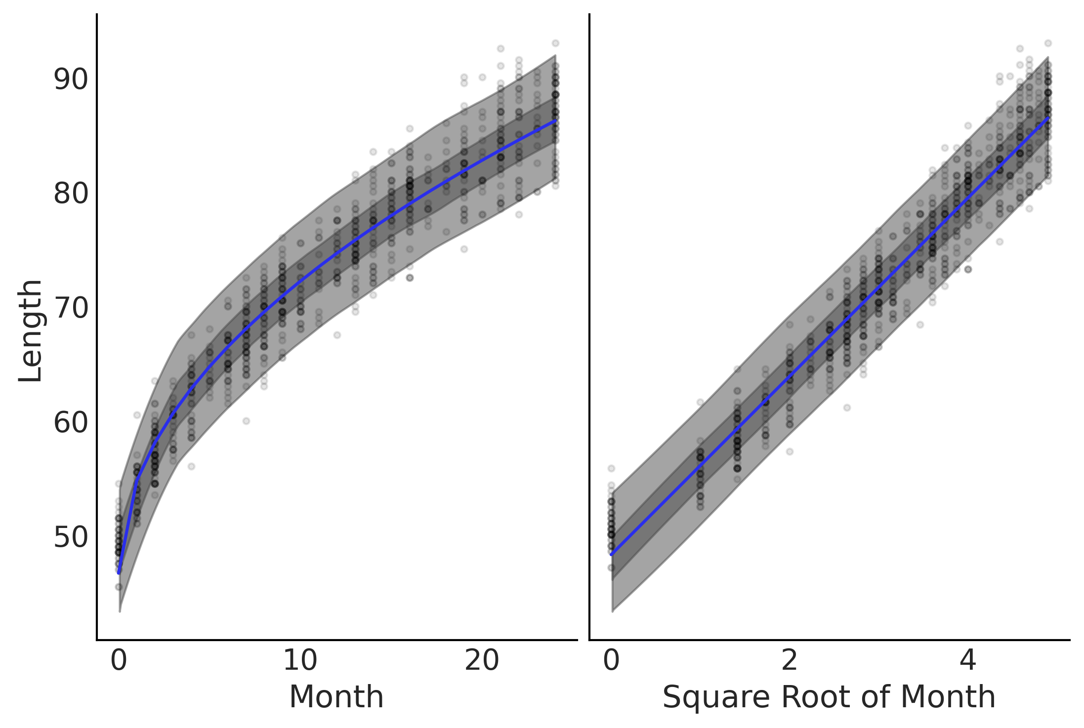
Figure 4.3

fig, axes = plt.subplots(1,2)
axes[0].plot(babies["Month"], babies["Length"], 'C0.', alpha=0.1)

μ_m = inf_data_sqrt.posterior["μ"].values.reshape(-1, babies["Length"].shape[0]).mean(axis=0)

axes[0].plot(babies["Month"], μ_m, c='C4')
az.plot_hdi(babies["Month"], inf_data_sqrt.posterior_predictive["length"], hdi_prob=.50, ax=axes[0])
az.plot_hdi(babies["Month"], inf_data_sqrt.posterior_predictive["length"], hdi_prob=.94, ax=axes[0])

axes[0].set_ylabel("Length")
axes[0].set_xlabel("Month");

axes[1].plot(np.sqrt(babies["Month"]), babies["Length"], 'C0.', alpha=0.1)
axes[1].set_xlabel("Square Root of Month");

az.plot_hdi(np.sqrt(babies["Month"]), inf_data_sqrt.posterior_predictive["length"], hdi_prob=.50, ax=axes[1])
az.plot_hdi(np.sqrt(babies["Month"]), inf_data_sqrt.posterior_predictive["length"], hdi_prob=.94, ax=axes[1])
axes[1].plot(np.sqrt(babies["Month"]), μ_m, c='C4')

axes[1].set_yticks([])
axes[1]

plt.savefig('img/chp04/baby_length_sqrt_fit.png', dpi=300)

az.compare({"Linear Model":inf_data_linear, "Non Linear Model":inf_data_sqrt})

/opt/miniconda3/envs/bmcp/lib/python3.9/site-packages/arviz/stats/stats.py:145: UserWarning: The default method used to estimate the weights for each model,has changed from BB-pseudo-BMA to stacking
  warnings.warn(

	rank	loo	p_loo	d_loo	weight	se	dse	warning	loo_scale
Non Linear Model	0	-1968.218405	3.079101	0.000000	0.928708	18.990940	0.000000	False	log
Linear Model	1	-2133.321593	3.229639	165.103188	0.071292	18.589207	20.083518	False	log

Varying Uncertainty

Code 4.4

with pm.Model() as model_baby_vv:
    β = pm.Normal("β", sigma=10, shape=2)

    # Additional variance terms
    δ = pm.HalfNormal("δ", sigma=10, shape=2)

    μ = pm.Deterministic("μ", β[0] + β[1] * np.sqrt(babies["Month"]))
    σ = pm.Deterministic("σ", δ[0] + δ[1] * babies["Month"])

    length = pm.Normal("length", mu=μ, sigma=σ, observed=babies["Length"])

    trace_baby_vv = pm.sample(2000, target_accept=.95)
    ppc_baby_vv = pm.sample_posterior_predictive(trace_baby_vv,
                                                 var_names=["length", "σ"])
    inf_data_baby_vv = az.from_pymc3(trace=trace_baby_vv,
                                     posterior_predictive=ppc_baby_vv)

/var/folders/7p/srk5qjp563l5f9mrjtp44bh800jqsw/T/ipykernel_8872/3065721124.py:12: FutureWarning: In v4.0, pm.sample will return an `arviz.InferenceData` object instead of a `MultiTrace` by default. You can pass return_inferencedata=True or return_inferencedata=False to be safe and silence this warning.
  trace_baby_vv = pm.sample(2000, target_accept=.95)
Auto-assigning NUTS sampler...
Initializing NUTS using jitter+adapt_diag...
Multiprocess sampling (4 chains in 4 jobs)
NUTS: [δ, β]

100.00% [12000/12000 00:09<00:00 Sampling 4 chains, 0 divergences]

Sampling 4 chains for 1_000 tune and 2_000 draw iterations (4_000 + 8_000 draws total) took 19 seconds.

100.00% [8000/8000 00:08<00:00]

az.summary(inf_data_baby_vv, var_names=["δ"])

	mean	sd	hdi_3%	hdi_97%	mcse_mean	mcse_sd	ess_bulk	ess_tail	r_hat
δ[0]	2.389	0.117	2.17	2.609	0.002	0.002	2715.0	2919.0	1.0
δ[1]	0.038	0.009	0.02	0.056	0.000	0.000	2663.0	2329.0	1.0

fig, ax = plt.subplots()

ax.set_ylabel("Length")
ax.set_xlabel("Month");

ax.plot(babies["Month"], babies["Length"], 'C0.', alpha=0.1)

μ_m = inf_data_baby_vv.posterior["μ"].values.reshape(-1, babies["Length"].shape[0]).mean(axis=0)

ax.plot(babies["Month"], μ_m, c='C4')

az.plot_hdi(babies["Month"], inf_data_baby_vv.posterior_predictive["length"], hdi_prob=.50, ax=ax)
az.plot_hdi(babies["Month"], inf_data_baby_vv.posterior_predictive["length"], hdi_prob=.94, ax=ax)

plt.savefig('img/chp04/baby_length_sqrt_vv_fit.png', dpi=300)

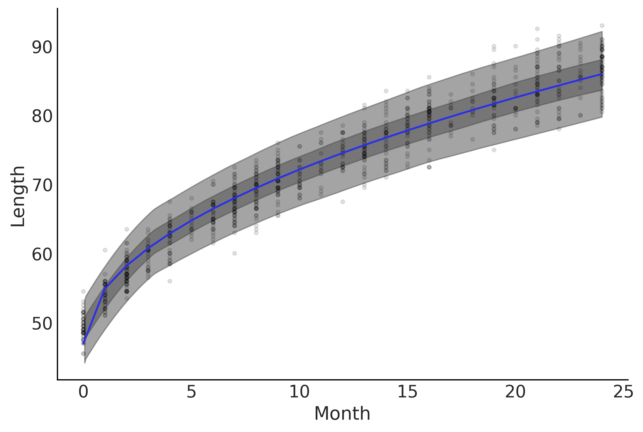
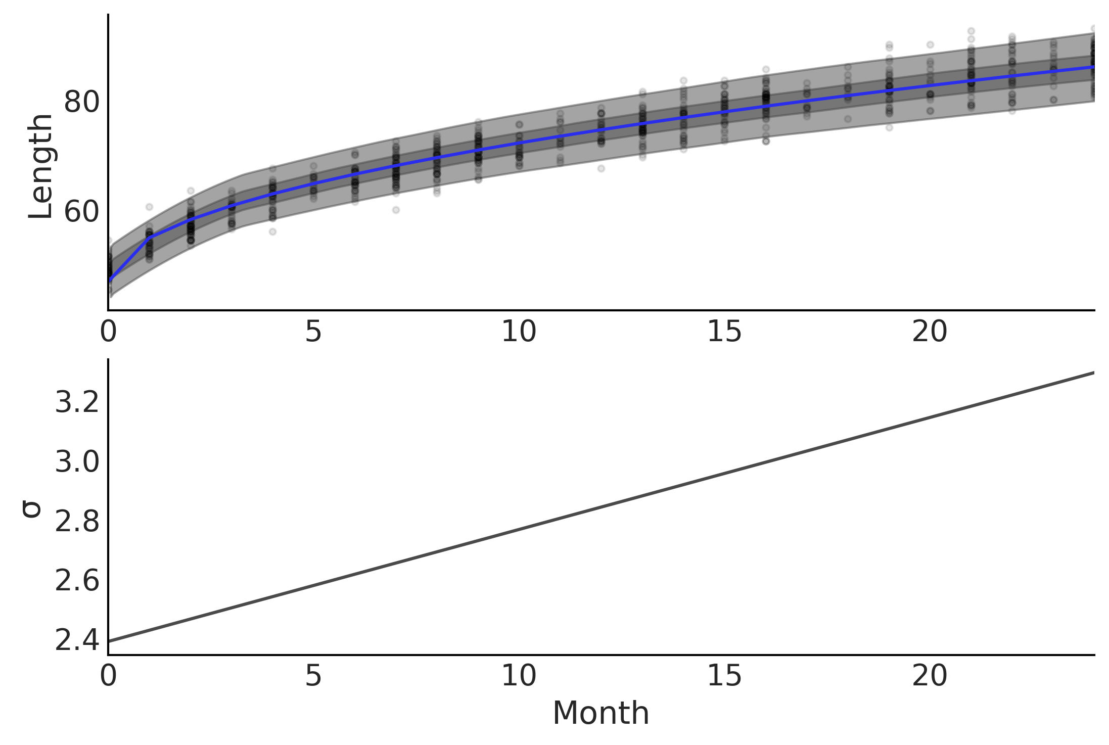
Figure 4.4

fig, axes = plt.subplots(2,1)

axes[0].plot(babies["Month"], babies["Length"], 'C0.', alpha=0.1)

μ_m = inf_data_baby_vv.posterior["μ"].values.reshape(-1, babies["Length"].shape[0]).mean(axis=0)

axes[0].plot(babies["Month"], μ_m, c='C4')

az.plot_hdi(babies["Month"], inf_data_baby_vv.posterior_predictive["length"], hdi_prob=.50, ax=axes[0])
az.plot_hdi(babies["Month"], inf_data_baby_vv.posterior_predictive["length"], hdi_prob=.94, ax=axes[0])
axes[0].set_ylabel("Length")

σ_m = inf_data_baby_vv.posterior["σ"].values.reshape(-1, 800).mean(axis=0)

axes[1].plot(babies["Month"], σ_m, c='C1')

axes[1].set_ylabel("σ")
axes[1].set_xlabel("Month")

axes[0].set_xlim(0,24)
axes[1].set_xlim(0,24)

plt.savefig('img/chp04/baby_length_sqrt_vv_fit_include_error.png', dpi=300)

Interaction effects

Code 4.5

tips_df = pd.read_csv('../data/tips.csv')
tips_df.head()

	total_bill	tip	sex	smoker	day	time	size
0	16.99	1.01	Female	No	Sun	Dinner	2
1	10.34	1.66	Male	No	Sun	Dinner	3
2	21.01	3.50	Male	No	Sun	Dinner	3
3	23.68	3.31	Male	No	Sun	Dinner	2
4	24.59	3.61	Female	No	Sun	Dinner	4

tips = tips_df["tip"]
total_bill_c = (tips_df["total_bill"] - tips_df["total_bill"].mean())  
smoker = pd.Categorical(tips_df["smoker"]).codes

with pm.Model() as model_no_interaction:
    β = pm.Normal("β", mu=0, sigma=1, shape=3)
    σ = pm.HalfNormal("σ", 1)

    μ = (β[0] +
         β[1] * total_bill_c + 
         β[2] * smoker)

    obs = pm.Normal("obs", μ, σ, observed=tips)
    trace_no_interaction = pm.sample(1000, tune=1000)

/var/folders/7p/srk5qjp563l5f9mrjtp44bh800jqsw/T/ipykernel_8872/3786948218.py:14: FutureWarning: In v4.0, pm.sample will return an `arviz.InferenceData` object instead of a `MultiTrace` by default. You can pass return_inferencedata=True or return_inferencedata=False to be safe and silence this warning.
  trace_no_interaction = pm.sample(1000, tune=1000)
Auto-assigning NUTS sampler...
Initializing NUTS using jitter+adapt_diag...
Multiprocess sampling (4 chains in 4 jobs)
NUTS: [σ, β]

100.00% [8000/8000 00:03<00:00 Sampling 4 chains, 0 divergences]

Sampling 4 chains for 1_000 tune and 1_000 draw iterations (4_000 + 4_000 draws total) took 13 seconds.

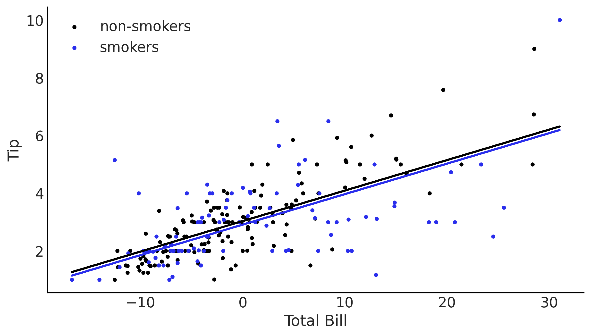
_, ax = plt.subplots(figsize=(8, 4.5))

β0_nonint = trace_no_interaction['β'][:,0]
β1_nonint = trace_no_interaction['β'][:,1]
β2_nonint = trace_no_interaction['β'][:,2]

pred_y_non_smokers = β0_nonint + β1_nonint * total_bill_c[:,None]
pred_y_smokers = β0_nonint + β1_nonint * total_bill_c[:,None] + β2_nonint

ax.scatter(total_bill_c[smoker==0], tips[smoker==0], label='non-smokers', marker='.')
ax.scatter(total_bill_c[smoker==1], tips[smoker==1], label='smokers', marker='.', c="C4")
ax.set_xlabel('Total Bill')
ax.set_ylabel('Tip')
ax.legend()

ax.plot(total_bill_c, pred_y_non_smokers.mean(1), lw=2)
ax.plot(total_bill_c, pred_y_smokers.mean(1), lw=2, c="C4");

/var/folders/7p/srk5qjp563l5f9mrjtp44bh800jqsw/T/ipykernel_8872/2436504886.py:7: FutureWarning: Support for multi-dimensional indexing (e.g. `obj[:, None]`) is deprecated and will be removed in a future version.  Convert to a numpy array before indexing instead.
  pred_y_non_smokers = β0_nonint + β1_nonint * total_bill_c[:,None]
/var/folders/7p/srk5qjp563l5f9mrjtp44bh800jqsw/T/ipykernel_8872/2436504886.py:8: FutureWarning: Support for multi-dimensional indexing (e.g. `obj[:, None]`) is deprecated and will be removed in a future version.  Convert to a numpy array before indexing instead.
  pred_y_smokers = β0_nonint + β1_nonint * total_bill_c[:,None] + β2_nonint

Code 4.6

with pm.Model() as model_interaction:
    β = pm.Normal('β', mu=0, sigma=1, shape=4)
    σ = pm.HalfNormal('σ', 1)

    μ = (β[0] +
         β[1] * total_bill_c + 
         β[2] * smoker +
         β[3] * smoker * total_bill_c
        )

    obs = pm.Normal('obs', μ, σ, observed=tips)
    trace_interaction = pm.sample(1000, tune=1000)

/var/folders/7p/srk5qjp563l5f9mrjtp44bh800jqsw/T/ipykernel_8872/146995100.py:12: FutureWarning: In v4.0, pm.sample will return an `arviz.InferenceData` object instead of a `MultiTrace` by default. You can pass return_inferencedata=True or return_inferencedata=False to be safe and silence this warning.
  trace_interaction = pm.sample(1000, tune=1000)
Auto-assigning NUTS sampler...
Initializing NUTS using jitter+adapt_diag...
Multiprocess sampling (4 chains in 4 jobs)
NUTS: [σ, β]

100.00% [8000/8000 00:04<00:00 Sampling 4 chains, 0 divergences]

Sampling 4 chains for 1_000 tune and 1_000 draw iterations (4_000 + 4_000 draws total) took 13 seconds.

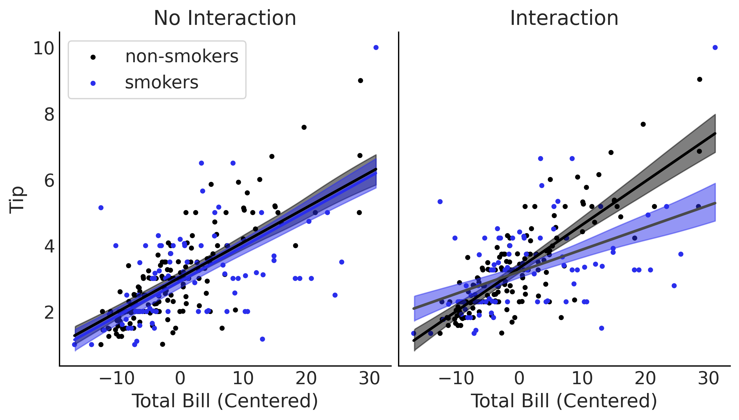
Figure 4.5

total_bill_c = total_bill_c.values

_, ax = plt.subplots(1, 2, figsize=(8, 4.5))

#α_nonint = trace_nonint['α']

β0_nonint = trace_no_interaction['β'][:,0]
β1_nonint = trace_no_interaction['β'][:,1]
β2_nonint = trace_no_interaction['β'][:,2]


pred_y_non_smokers = β0_nonint + β1_nonint * total_bill_c[:,None]
pred_y_smokers = β0_nonint + β1_nonint * total_bill_c[:,None] + β2_nonint

ax[0].scatter(total_bill_c[smoker==0], tips[smoker==0], label='non-smokers', marker='.')
ax[0].scatter(total_bill_c[smoker==1], tips[smoker==1], label='smokers', marker='.', c="C4")
ax[0].set_xlabel('Total Bill (Centered)')
ax[0].set_ylabel('Tip')
ax[0].legend(frameon=True)

ax[0].plot(total_bill_c, pred_y_non_smokers.mean(1), lw=2)
ax[0].plot(total_bill_c, pred_y_smokers.mean(1), lw=2, c="C4")
ax[0].set_title('No Interaction')


az.plot_hdi(total_bill_c, pred_y_non_smokers.T, color='C0', ax=ax[0])
az.plot_hdi(total_bill_c, pred_y_smokers.T, ax=ax[0], color="C4");

β0_int = trace_interaction['β'][:,0]
β1_int = trace_interaction['β'][:,1]
β2_int = trace_interaction['β'][:,2]
β3_int = trace_interaction['β'][:,3]

# Because smoker=0 I am ommiting the terms including the smoker covariate
pred_y_non_smokers = (β0_int +
                      β1_int * total_bill_c[:, None])

# Because x1=1 I am ommiting x1
pred_y_smokers = (β0_int +
                  β1_int * total_bill_c[:, None] +
                  β2_int +
                  β3_int * total_bill_c[:, None])


ax[1].scatter(total_bill_c[smoker==0], tips[smoker==0], label='non-smokers', marker='.')
ax[1].scatter(total_bill_c[smoker==1], tips[smoker==1], label='smokers', marker='.', c="C4")
ax[1].set_xlabel('Total Bill (Centered)')
ax[1].set_yticks([])

ax[1].set_title('Interaction')

ax[1].plot(total_bill_c, pred_y_non_smokers.mean(1), lw=2)
ax[1].plot(total_bill_c, pred_y_smokers.mean(1), lw=2)
az.plot_hdi(total_bill_c, pred_y_non_smokers.T, color='C0', ax=ax[1])
az.plot_hdi(total_bill_c, pred_y_smokers.T, ax=ax[1], color="C4");

plt.savefig('img/chp04/smoker_tip_interaction.png', dpi=300)

/opt/miniconda3/envs/bmcp/lib/python3.9/site-packages/arviz/stats/stats.py:456: FutureWarning: hdi currently interprets 2d data as (draw, shape) but this will change in a future release to (chain, draw) for coherence with other functions
  warnings.warn(
/opt/miniconda3/envs/bmcp/lib/python3.9/site-packages/arviz/stats/stats.py:456: FutureWarning: hdi currently interprets 2d data as (draw, shape) but this will change in a future release to (chain, draw) for coherence with other functions
  warnings.warn(
/opt/miniconda3/envs/bmcp/lib/python3.9/site-packages/arviz/stats/stats.py:456: FutureWarning: hdi currently interprets 2d data as (draw, shape) but this will change in a future release to (chain, draw) for coherence with other functions
  warnings.warn(
/opt/miniconda3/envs/bmcp/lib/python3.9/site-packages/arviz/stats/stats.py:456: FutureWarning: hdi currently interprets 2d data as (draw, shape) but this will change in a future release to (chain, draw) for coherence with other functions
  warnings.warn(

Robust Regression

Figure 4.6

mean = 5
sigma = 2

x = np.linspace(-5, 15, 1000)
fig, ax = plt.subplots()

ax.plot(x, stats.norm(5,2).pdf(x), label=f"Normal μ={mean}, σ={sigma}", color="C4")

for i, nu in enumerate([1, 2, 20],1):
    ax.plot(x, stats.t(loc=5, scale=2, df=nu).pdf(x), label=f"Student T μ={mean}, σ={sigma}, ν={nu}", color=f"C{i}")

ax.set_xlim(-5, 18)
ax.legend(loc="upper right", frameon=False)
ax.set_yticks([])
plt.savefig('img/chp04/studentt_normal_comparison.png', dpi=300)

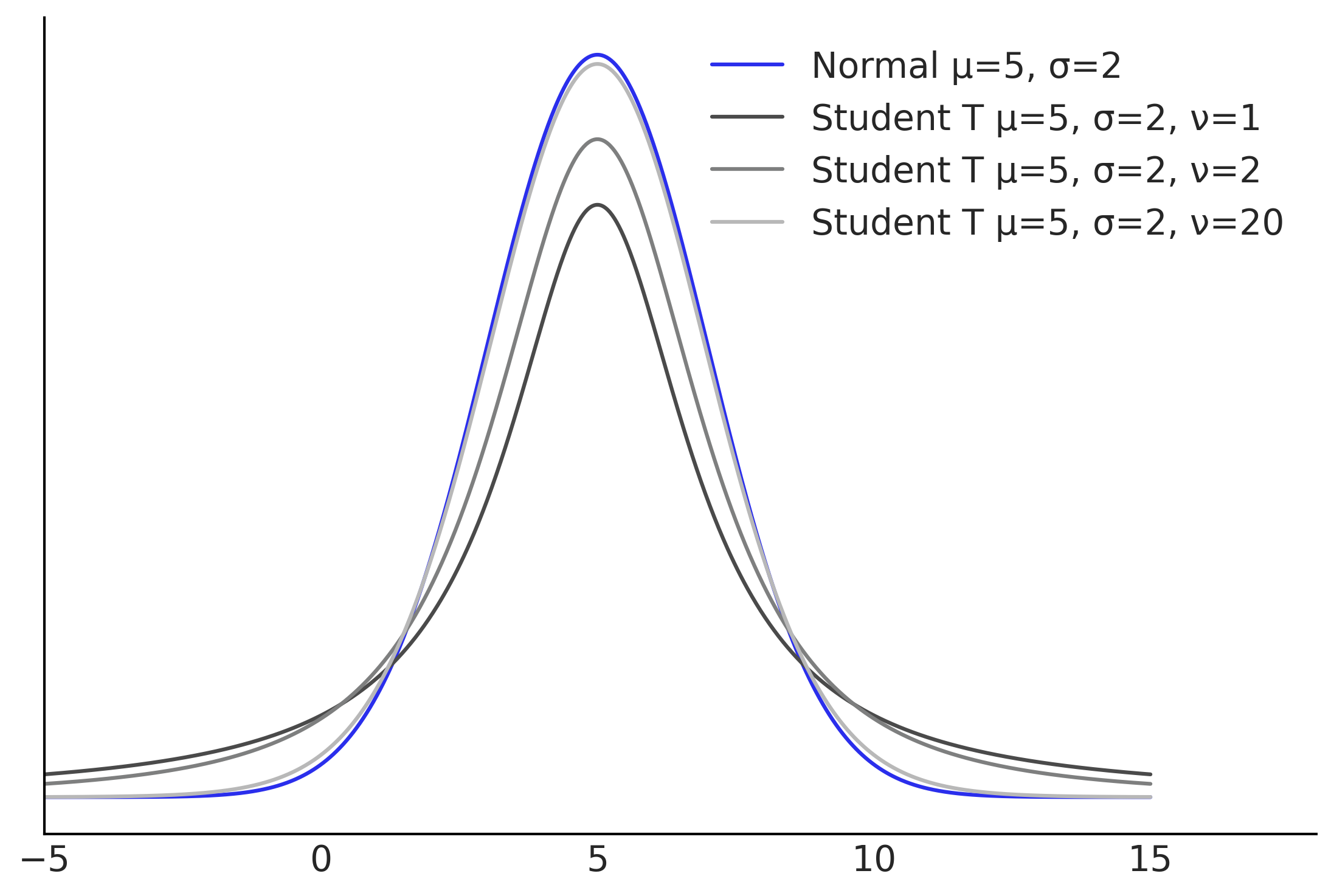
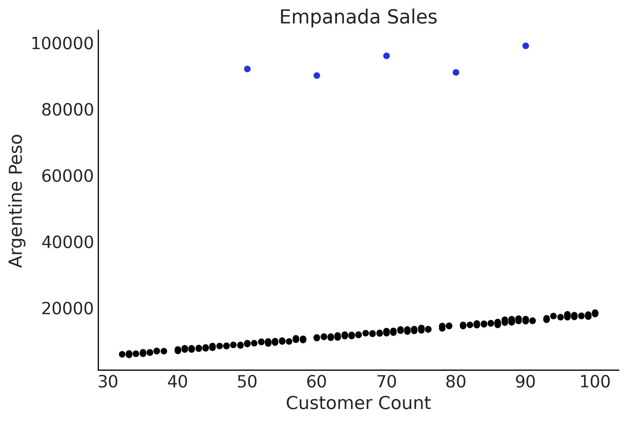
Figure 4.7

def generate_sales(*, days, mean, std, label):
    np.random.seed(0)
    df = pd.DataFrame(index=range(1, days+1), columns=["customers", "sales"])
    for day in range(1, days+1):
        num_customers = stats.randint(30, 100).rvs()+1
        
        # This is correct as there is an independent draw for each customers orders
        dollar_sales = stats.norm(mean, std).rvs(num_customers).sum()
        
        df.loc[day, "customers"] = num_customers
        df.loc[day, "sales"] = dollar_sales
        
    # Fix the types as not to cause Theano errors
    df = df.astype({'customers': 'int32', 'sales': 'float32'})
    
    # Sorting will make plotting the posterior predictive easier later
    df["Food_Category"] = label
    df = df.sort_values("customers")
    return df

fig, ax = plt.subplots()

empanadas =  generate_sales(days=200, mean=180, std=30, label="Empanada")
empanadas.iloc[0] = [50, 92000, "Empanada"]
empanadas.iloc[1] = [60, 90000, "Empanada"]
empanadas.iloc[2] = [70, 96000, "Empanada"]
empanadas.iloc[3] = [80, 91000, "Empanada"]
empanadas.iloc[4] = [90, 99000, "Empanada"]

empanadas = empanadas.sort_values("customers")

empanadas.sort_values("sales")[:-5].plot(x="customers", y="sales", kind="scatter", ax=ax);
empanadas.sort_values("sales")[-5:].plot(x="customers", y="sales", kind="scatter", c="C4", ax=ax);

ax.set_ylabel("Argentine Peso")
ax.set_xlabel("Customer Count")
ax.set_title("Empanada Sales")
plt.savefig('img/chp04/empanada_scatter_plot.png', dpi=300)

Code 4.7

with pm.Model() as model_non_robust:
    σ = pm.HalfNormal("σ", 50)
    β = pm.Normal('β', mu=150, sigma=20)

    μ = pm.Deterministic("μ", β * empanadas["customers"])
    
    sales = pm.Normal("sales", mu=μ, sigma=σ, observed=empanadas["sales"])
    
    trace_empanada_sales = pm.sample(random_seed=1)
    ppc_empanada_sales = pm.sample_posterior_predictive(
        trace_empanada_sales)
    inf_data_non_robust = az.from_pymc3(trace = trace_empanada_sales,
                                        posterior_predictive=ppc_empanada_sales)

/var/folders/7p/srk5qjp563l5f9mrjtp44bh800jqsw/T/ipykernel_8872/1588961933.py:9: FutureWarning: In v4.0, pm.sample will return an `arviz.InferenceData` object instead of a `MultiTrace` by default. You can pass return_inferencedata=True or return_inferencedata=False to be safe and silence this warning.
  trace_empanada_sales = pm.sample(random_seed=1)
Auto-assigning NUTS sampler...
Initializing NUTS using jitter+adapt_diag...
Multiprocess sampling (4 chains in 4 jobs)
NUTS: [β, σ]

100.00% [8000/8000 00:07<00:00 Sampling 4 chains, 0 divergences]

Sampling 4 chains for 1_000 tune and 1_000 draw iterations (4_000 + 4_000 draws total) took 16 seconds.
The acceptance probability does not match the target. It is 0.8860777877942666, but should be close to 0.8. Try to increase the number of tuning steps.

100.00% [4000/4000 00:03<00:00]

Figure 4.8

fig, axes = plt.subplots(2, 1, figsize=(8, 4), sharex=True)
μ_m = inf_data_non_robust.posterior["μ"].values.reshape(-1, empanadas.shape[0]).mean(axis=0)

for i in range(2):
    empanadas.sort_values("sales")[:-5].plot(x="customers", y="sales", kind="scatter", ax=axes[i]);
    empanadas.sort_values("sales")[-5:].plot(x="customers", y="sales", kind="scatter", c="C4", ax=axes[i]);
    axes[i].plot(empanadas.customers, μ_m, c='C4')
    az.plot_hdi(empanadas.customers, inf_data_non_robust.posterior_predictive["sales"], hdi_prob=.95, ax=axes[i])

    axes[1].set_ylabel("Argentine Peso")

axes[0].set_ylabel("")
axes[1].set_xlabel("Customer Count")
axes[1].set_ylim(400, 25000);
plt.savefig('img/chp04/empanada_scatter_non_robust.png', dpi=300)

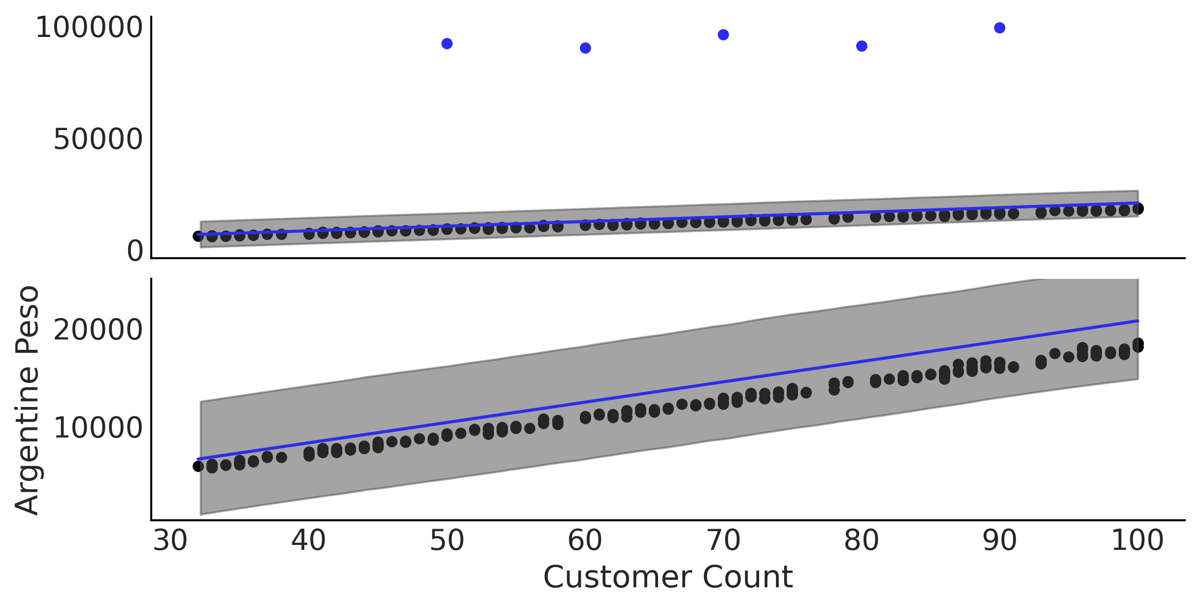
Table 4.1

az.summary(inf_data_non_robust, kind="stats", var_names=["β", "σ"]).round(1)

	mean	sd	hdi_3%	hdi_97%
β	207.0	3.0	201.4	212.5
σ	2952.3	25.3	2904.3	2997.6

with pm.Model() as model_robust:
    σ = pm.HalfNormal("σ", 50)
    β = pm.Normal("β", mu=150, sigma=20)
    ν = pm.HalfNormal("ν", 20)

    μ = pm.Deterministic("μ", β * empanadas["customers"])
    
    sales = pm.StudentT("sales", mu=μ, sigma=σ, nu=ν,
                        observed=empanadas["sales"])
        
    trace_empanada_sales_robust = pm.sample(random_seed=0)
    ppc_empanada_sales_robust = pm.sample_posterior_predictive(
                                        trace_empanada_sales_robust)
    
    inf_data_robust = az.from_pymc3(trace = trace_empanada_sales_robust,
                                    posterior_predictive=ppc_empanada_sales_robust)

/var/folders/7p/srk5qjp563l5f9mrjtp44bh800jqsw/T/ipykernel_8872/2239246076.py:11: FutureWarning: In v4.0, pm.sample will return an `arviz.InferenceData` object instead of a `MultiTrace` by default. You can pass return_inferencedata=True or return_inferencedata=False to be safe and silence this warning.
  trace_empanada_sales_robust = pm.sample(random_seed=0)
Auto-assigning NUTS sampler...
Initializing NUTS using jitter+adapt_diag...
Multiprocess sampling (4 chains in 4 jobs)
NUTS: [ν, β, σ]

100.00% [8000/8000 00:03<00:00 Sampling 4 chains, 0 divergences]

Sampling 4 chains for 1_000 tune and 1_000 draw iterations (4_000 + 4_000 draws total) took 12 seconds.

100.00% [4000/4000 00:02<00:00]

Table 4.2

az.summary(inf_data_robust, var_names=["β", "σ", "ν"], kind="stats").round(1)

	mean	sd	hdi_3%	hdi_97%
β	179.6	0.3	179.1	180.1
σ	152.0	13.9	126.4	178.4
ν	1.3	0.2	1.0	1.6

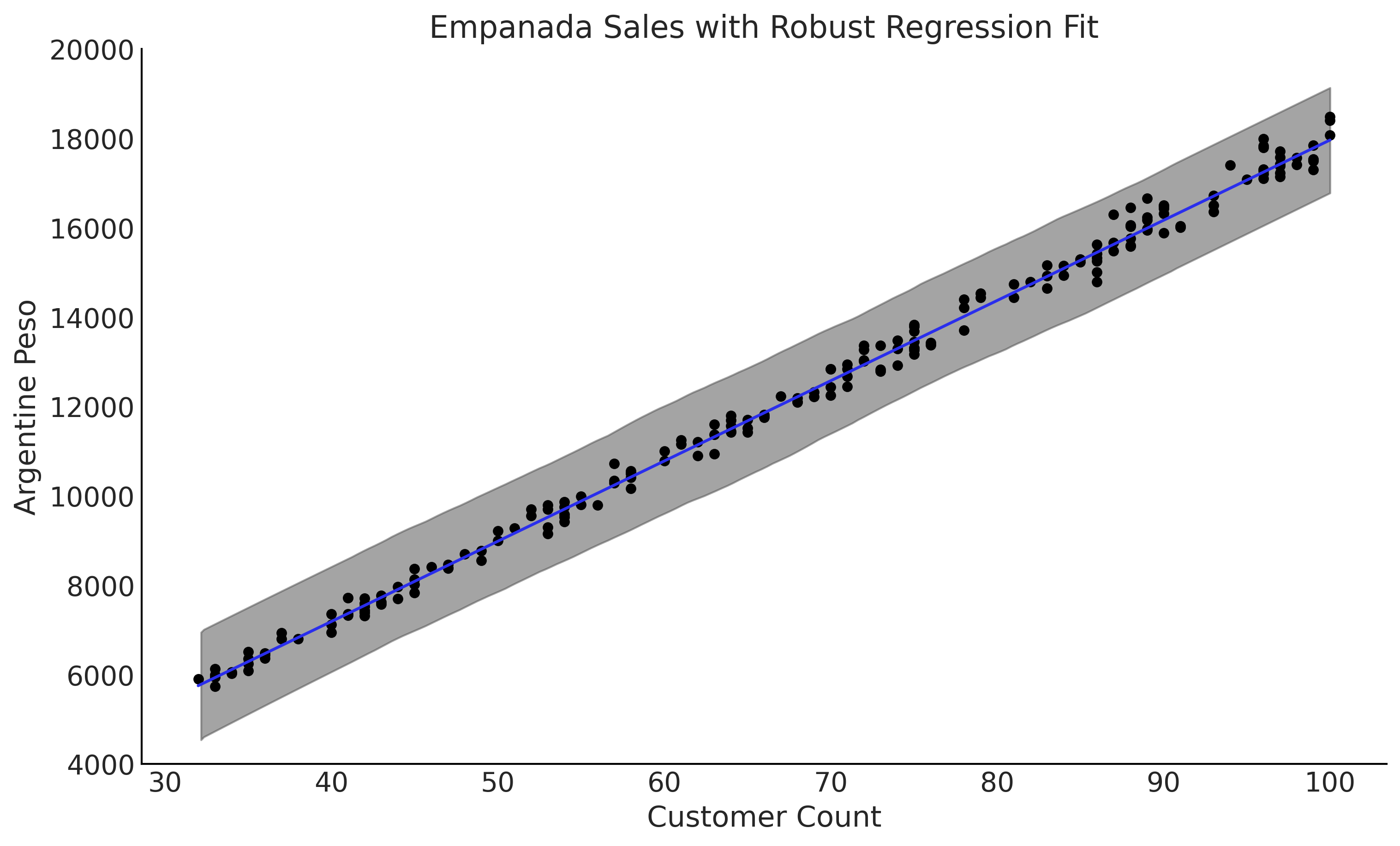
Figure 4.9

fig, ax = plt.subplots(figsize=(10, 6))
μ_m = inf_data_robust.posterior["μ"].values.reshape(-1, empanadas.shape[0]).mean(axis=0)

ax.plot(empanadas.customers, μ_m, c='C4')
az.plot_hdi(empanadas.customers, inf_data_robust.posterior_predictive["sales"], hdi_prob=.95, ax=ax)

empanadas.plot(x="customers", y="sales", kind="scatter", ax=ax)
ax.set_ylim(4000, 20000);
ax.set_ylabel("Argentine Peso")
ax.set_xlabel("Customer Count")
ax.set_title("Empanada Sales with Robust Regression Fit")
plt.savefig('img/chp04/empanada_scatter_robust.png', dpi=300)

az.compare({"Non robust": inf_data_non_robust, "Robust":inf_data_robust})

/opt/miniconda3/envs/bmcp/lib/python3.9/site-packages/arviz/stats/stats.py:145: UserWarning: The default method used to estimate the weights for each model,has changed from BB-pseudo-BMA to stacking
  warnings.warn(
/opt/miniconda3/envs/bmcp/lib/python3.9/site-packages/arviz/stats/stats.py:655: UserWarning: Estimated shape parameter of Pareto distribution is greater than 0.7 for one or more samples. You should consider using a more robust model, this is because importance sampling is less likely to work well if the marginal posterior and LOO posterior are very different. This is more likely to happen with a non-robust model and highly influential observations.
  warnings.warn(

	rank	loo	p_loo	d_loo	weight	se	dse	warning	loo_scale
Robust	0	-1473.978565	5.912134	0.000000	1.000000e+00	31.902351	0.000000	False	log
Non robust	1	-3698.588569	146.177400	2224.610004	1.146134e-09	829.237992	799.490297	True	log

Pooling, Multilevel Models, and Mixed Effects

def generate_sales(*, days, mean, std, label):
    np.random.seed(0)
    df = pd.DataFrame(index=range(1, days+1), columns=["customers", "sales"])
    for day in range(1, days+1):
        num_customers = stats.randint(30, 100).rvs()+1
        
        # This is correct as there is an independent draw for each customers orders
        dollar_sales = stats.norm(mean, std).rvs(num_customers).sum()
        
        df.loc[day, "customers"] = num_customers
        df.loc[day, "sales"] = dollar_sales
        
    # Fix the types as not to cause Theano errors
    df = df.astype({'customers': 'int32', 'sales': 'float32'})
    
    # Sorting will make plotting the posterior predictive easier later
    df["Food_Category"] = label
    df = df.sort_values("customers")
    return df

pizza_df = generate_sales(days=365, mean=13, std=5, label="Pizza")
sandwich_df = generate_sales(days=100, mean=6, std=5, label="Sandwich")

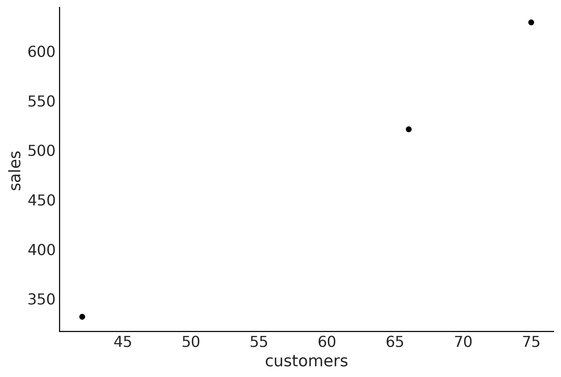
salad_days = 3
salad_df = generate_sales(days=salad_days, mean=8 ,std=3, label="Salad")

salad_df.plot(x="customers", y="sales", kind="scatter");

sales_df = pd.concat([pizza_df, sandwich_df, salad_df]).reset_index(drop=True)
sales_df["Food_Category"] = pd.Categorical(sales_df["Food_Category"])
sales_df

	customers	sales	Food_Category
0	31	459.895203	Pizza
1	31	401.147736	Pizza
2	31	413.345245	Pizza
3	31	371.909241	Pizza
4	32	433.797089	Pizza
...	...	...	...
463	100	611.736816	Sandwich
464	100	667.152954	Sandwich
465	42	331.625702	Salad
466	66	520.900940	Salad
467	75	628.937622	Salad

468 rows × 3 columns

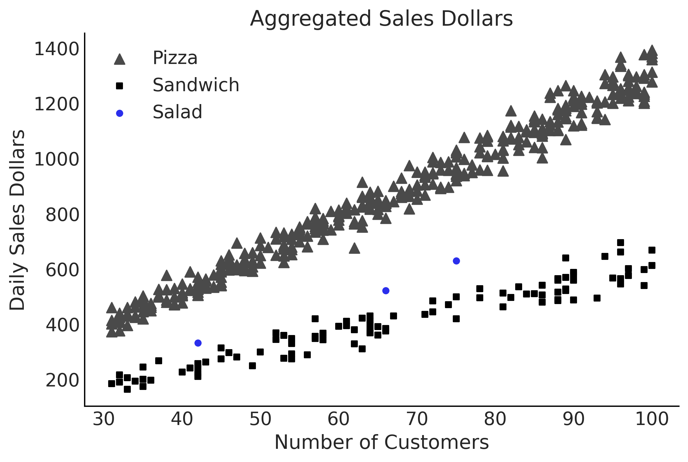
Figure 4.10

fig, ax = plt.subplots()
pizza_df.plot(x="customers", y="sales", kind="scatter", ax=ax, c="C1", label="Pizza", marker="^", s=60);
sandwich_df.plot(x="customers", y="sales", kind="scatter", ax=ax,  label="Sandwich", marker="s");
salad_df.plot(x="customers", y="sales", kind="scatter", ax=ax, label="Salad", c="C4");

ax.set_xlabel("Number of Customers")
ax.set_ylabel("Daily Sales Dollars")
ax.set_title("Aggregated Sales Dollars")
ax.legend()

plt.savefig('img/chp04/restaurant_order_scatter.png', dpi=300)

Unpooled Model

Code 4.9

customers = sales_df.loc[:, "customers"].values
sales_observed = sales_df.loc[:, "sales"].values
food_category = pd.Categorical(sales_df["Food_Category"])

with pm.Model() as model_sales_unpooled:
    σ = pm.HalfNormal("σ", 20, shape=3)
    β = pm.Normal("β", mu=10, sigma=10, shape=3)
    
    μ = pm.Deterministic("μ", β[food_category.codes] *customers)
    
    sales = pm.Normal("sales", mu=μ, sigma=σ[food_category.codes],
                      observed=sales_observed)
    
    trace_sales_unpooled = pm.sample(target_accept=.9)
    inf_data_sales_unpooled = az.from_pymc3(
        trace=trace_sales_unpooled, 
        coords={"β_dim_0":food_category.categories,
                "σ_dim_0":food_category.categories})

/var/folders/7p/srk5qjp563l5f9mrjtp44bh800jqsw/T/ipykernel_8872/3049063767.py:14: FutureWarning: In v4.0, pm.sample will return an `arviz.InferenceData` object instead of a `MultiTrace` by default. You can pass return_inferencedata=True or return_inferencedata=False to be safe and silence this warning.
  trace_sales_unpooled = pm.sample(target_accept=.9)
Auto-assigning NUTS sampler...
Initializing NUTS using jitter+adapt_diag...
Multiprocess sampling (4 chains in 4 jobs)
NUTS: [β, σ]

100.00% [8000/8000 00:05<00:00 Sampling 4 chains, 0 divergences]

Sampling 4 chains for 1_000 tune and 1_000 draw iterations (4_000 + 4_000 draws total) took 14 seconds.

Figure 4.12

sales_unpooled_diagram = pm.model_to_graphviz(model_sales_unpooled)
sales_unpooled_diagram.render("img/chp04/salad_sales_basic_regression_model_unpooled", format="png", cleanup=True)
sales_unpooled_diagram

inf_data_salads_sales_unpooled = inf_data_sales_unpooled.posterior.sel(β_dim_0="Salad", μ_dim_0=slice(465, 467))

az.summary(inf_data_sales_unpooled, var_names=["β", "σ"])

	mean	sd	hdi_3%	hdi_97%	mcse_mean	mcse_sd	ess_bulk	ess_tail	r_hat
β[0]	13.025	0.030	12.970	13.081	0.000	0.000	5104.0	2785.0	1.0
β[1]	8.129	0.214	7.720	8.561	0.004	0.003	3504.0	2280.0	1.0
β[2]	6.111	0.052	6.010	6.204	0.001	0.001	5298.0	2765.0	1.0
σ[0]	40.128	1.469	37.362	42.801	0.020	0.014	5405.0	2605.0	1.0
σ[1]	21.361	8.327	8.919	37.105	0.158	0.116	3148.0	3021.0	1.0
σ[2]	35.931	2.506	31.092	40.501	0.034	0.024	5377.0	2902.0	1.0

az.plot_trace(inf_data_sales_unpooled, var_names=["β", "σ"], compact=False);

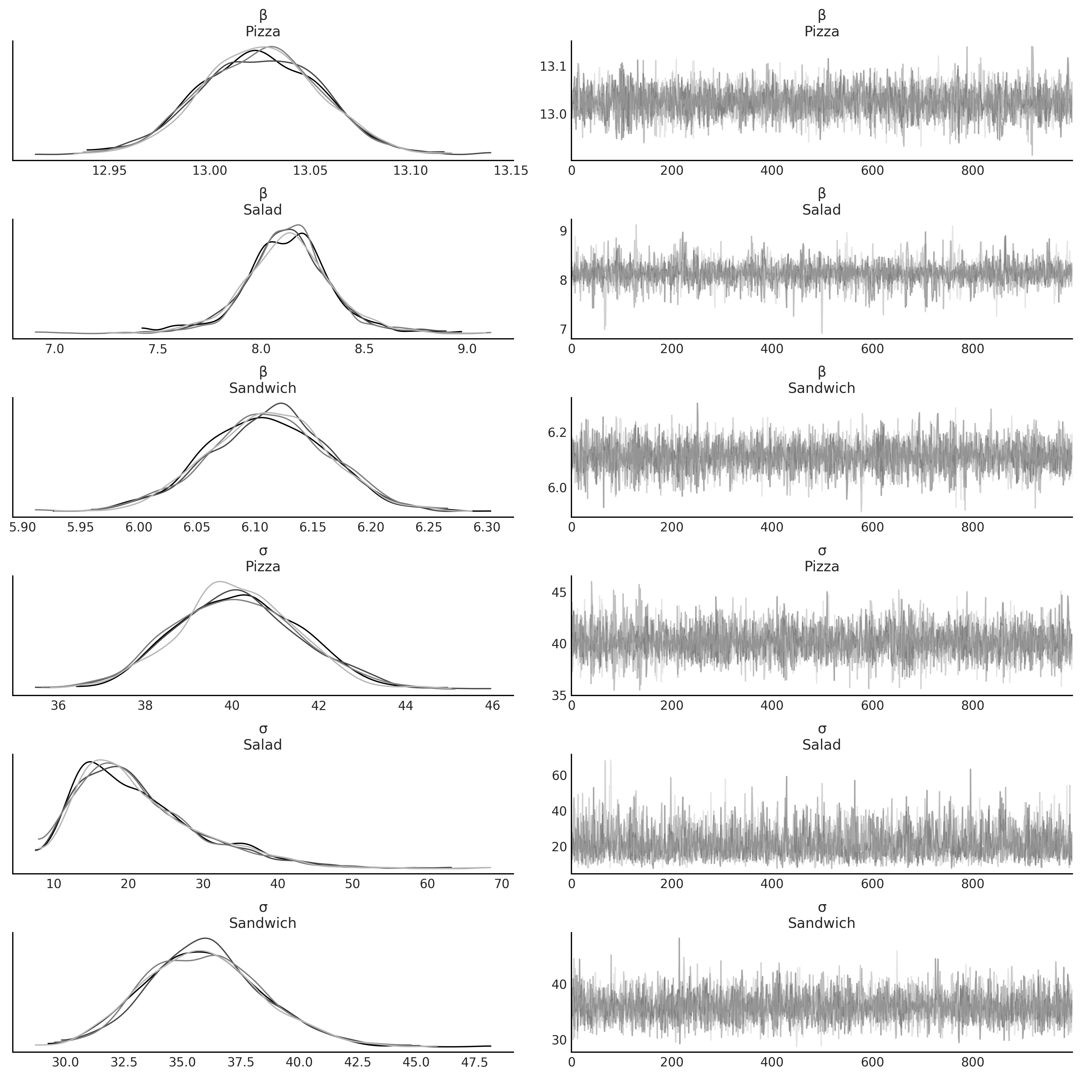
Figure 4.13

axes = az.plot_forest([inf_data_sales_unpooled],
                      model_names = ["Unpooled",],
                      var_names=["β"], combined=True, figsize=(7, 1.8));
axes[0].set_title("β parameter estimates 94% HDI")
plt.savefig("img/chp04/salad_sales_basic_regression_forestplot_beta.png")

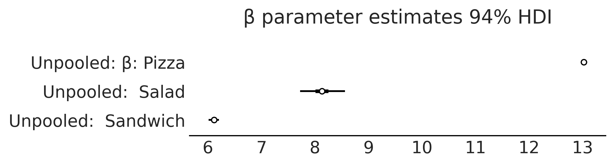
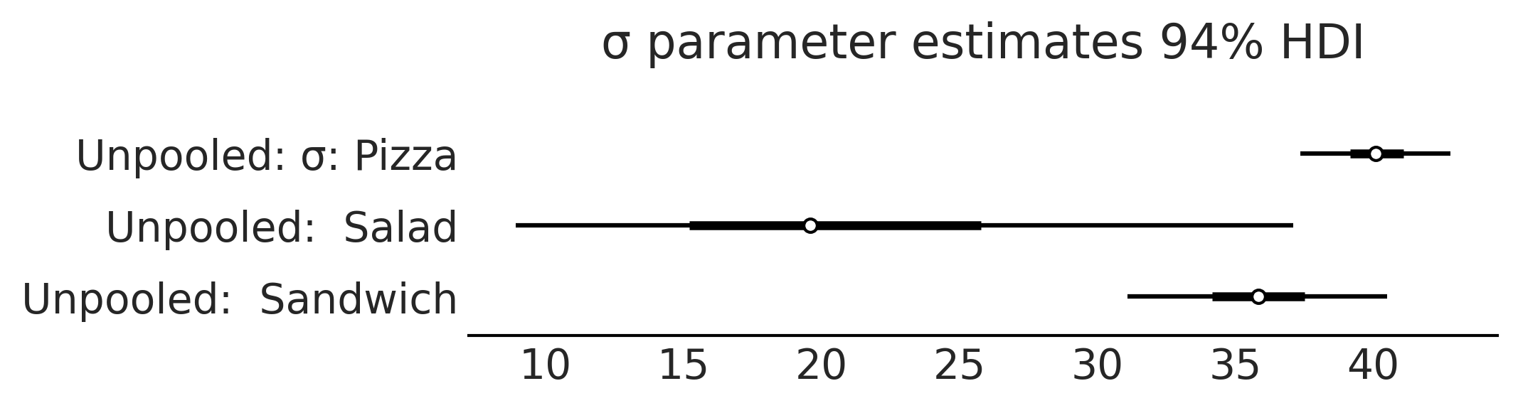
Figure 4.14

axes = az.plot_forest([inf_data_salads_sales_unpooled,],
                      model_names = ["Unpooled",],
                      var_names=["σ"], combined=True, figsize=(7, 1.8));
axes[0].set_title("σ parameter estimates 94% HDI")
plt.savefig("img/chp04/salad_sales_basic_regression_forestplot_sigma.png")

Pooled Model

Code 4.10

with pm.Model() as model_sales_pooled:
    σ = pm.HalfNormal("σ", 20)
    β = pm.Normal("β", mu=10, sigma=10)

    μ = pm.Deterministic("μ", β * customers)
    
    sales = pm.Normal("sales", mu=μ, sigma=σ,
                      observed=sales_observed)
                        
    inf_data_sales_pooled = pm.sample()

/var/folders/7p/srk5qjp563l5f9mrjtp44bh800jqsw/T/ipykernel_8872/1895007518.py:10: FutureWarning: In v4.0, pm.sample will return an `arviz.InferenceData` object instead of a `MultiTrace` by default. You can pass return_inferencedata=True or return_inferencedata=False to be safe and silence this warning.
  inf_data_sales_pooled = pm.sample()
Auto-assigning NUTS sampler...
Initializing NUTS using jitter+adapt_diag...
Multiprocess sampling (4 chains in 4 jobs)
NUTS: [β, σ]

100.00% [8000/8000 00:02<00:00 Sampling 4 chains, 0 divergences]

Sampling 4 chains for 1_000 tune and 1_000 draw iterations (4_000 + 4_000 draws total) took 11 seconds.

with model_sales_pooled:
    ppc_sales_pooled = pm.sample_posterior_predictive(inf_data_sales_pooled)
    inf_data_sales_pooled = az.from_pymc3(
        trace=inf_data_sales_pooled,
        posterior_predictive=ppc_sales_pooled)

100.00% [4000/4000 00:03<00:00]

Figure 4.16

pooled_sales_diagram = pm.model_to_graphviz(model_sales_pooled)
pooled_sales_diagram.render("img/chp04/salad_sales_basic_regression_model_pooled", format="png", cleanup=True)
pooled_sales_diagram

az.plot_trace(inf_data_sales_pooled, var_names=["β", "σ"], compact=False);

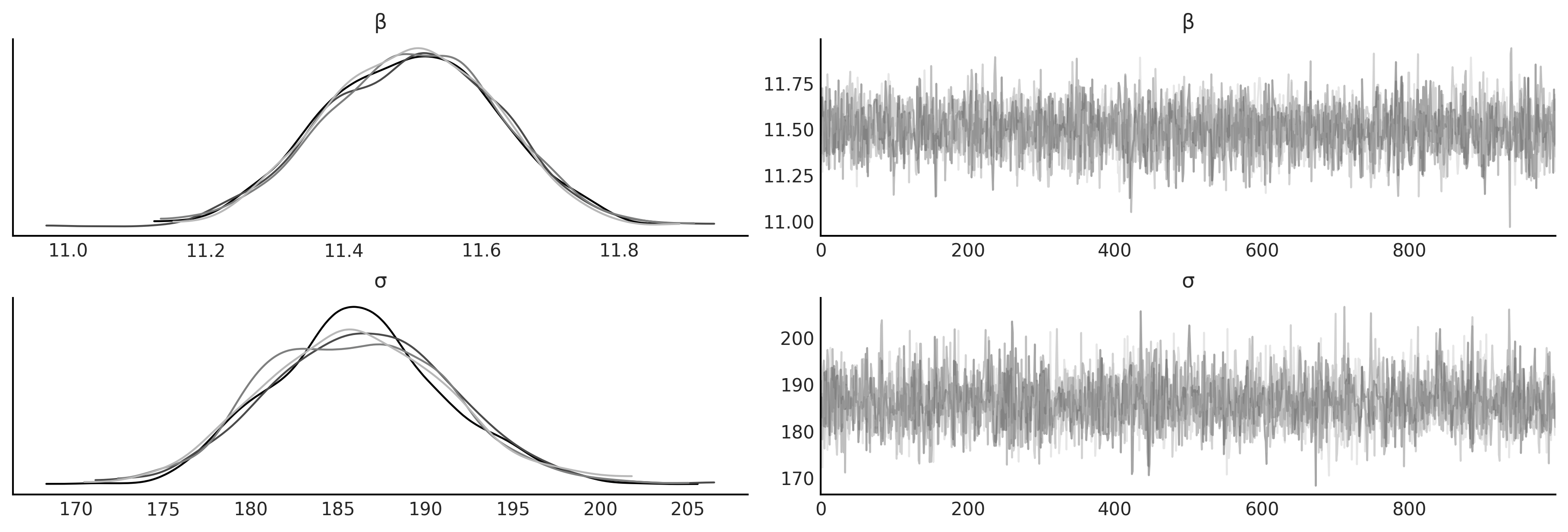
az.summary(inf_data_sales_pooled, var_names=["β", "σ"])

	mean	sd	hdi_3%	hdi_97%	mcse_mean	mcse_sd	ess_bulk	ess_tail	r_hat
β	11.498	0.126	11.264	11.729	0.002	0.001	3561.0	2629.0	1.0
σ	186.204	5.271	176.336	195.841	0.090	0.063	3466.0	3240.0	1.0

Figure 4.17

axes = az.plot_forest([inf_data_sales_pooled, inf_data_sales_unpooled],
                      model_names = ["Pooled", "Unpooled"], var_names=["σ"], combined=True, figsize=(7, 1.8));
axes[0].set_title("Comparison of pooled and unpooled models \n 94% HDI")

#plt.subplots_adjust(top=1)
plt.savefig("img/chp04/salad_sales_basic_regression_forestplot_sigma_comparison.png", bbox_inches='tight')

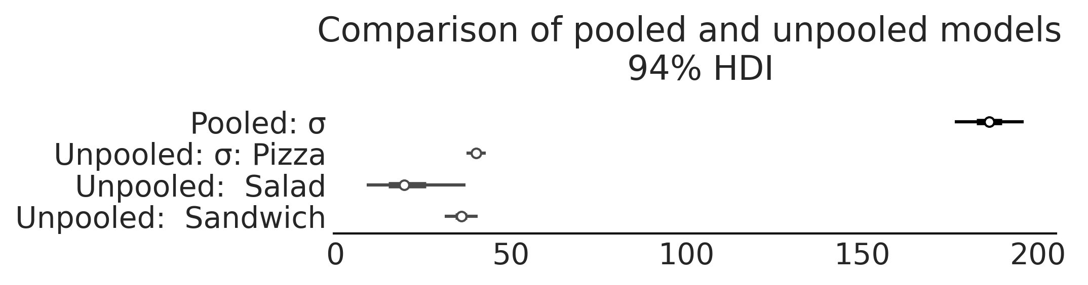
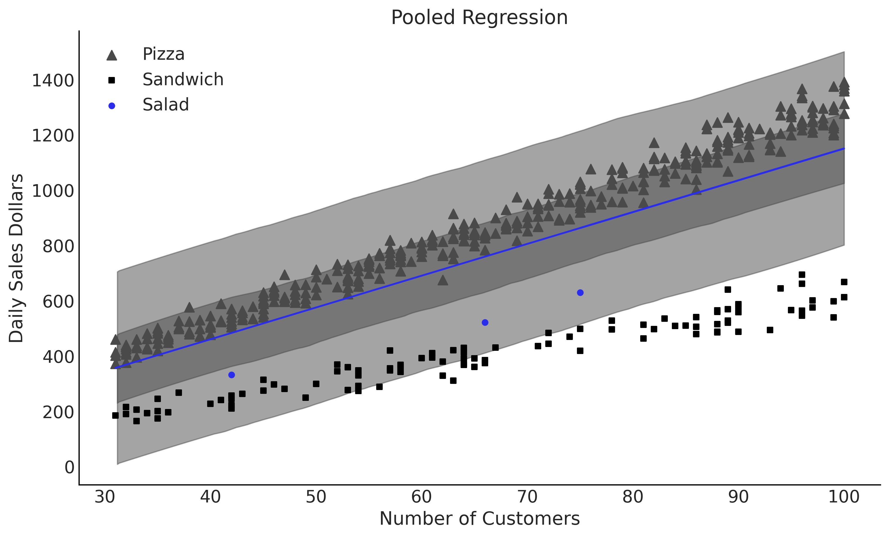
Figure 4.18

fig, ax = plt.subplots(figsize=(10, 6))
μ_m = inf_data_sales_pooled.posterior["μ"].values.reshape(-1, sales_df.shape[0]).mean(axis=0)
σ_m = inf_data_sales_pooled.posterior["σ"].mean().values

ax.plot(customers, μ_m, c='C4')

az.plot_hdi(customers, inf_data_sales_pooled.posterior_predictive["sales"], hdi_prob=.50, ax=ax)
az.plot_hdi(customers, inf_data_sales_pooled.posterior_predictive["sales"], hdi_prob=.94, ax=ax)


pizza_df.plot(x="customers", y="sales", kind="scatter", ax=ax, c="C1", label="Pizza", marker="^", s=60);
sandwich_df.plot(x="customers", y="sales", kind="scatter", ax=ax,  label="Sandwich", marker="s");
salad_df.plot(x="customers", y="sales", kind="scatter", ax=ax, label="Salad", c="C4");


ax.set_xlabel("Number of Customers")
ax.set_ylabel("Daily Sales Dollars")
ax.set_title("Pooled Regression")
plt.savefig("img/chp04/salad_sales_basic_regression_scatter_pooled.png")

Code 4.11

with pm.Model() as model_pooled_sigma_sales:
    σ = pm.HalfNormal("σ", 20)
    β = pm.Normal("β", mu=10, sigma=20, shape=3)
    
    μ = pm.Deterministic("μ", β[food_category.codes] * customers)
    
    sales = pm.Normal("sales", mu=μ, sigma=σ, observed=sales_observed)
    
    trace_pooled_sigma_sales = pm.sample()
    ppc_pooled_sigma_sales = pm.sample_posterior_predictive(
        trace_pooled_sigma_sales)

    inf_data_pooled_sigma_sales = az.from_pymc3(
        trace=trace_pooled_sigma_sales,
        posterior_predictive=ppc_pooled_sigma_sales,
        coords={"β_dim_0":food_category.categories})

/var/folders/7p/srk5qjp563l5f9mrjtp44bh800jqsw/T/ipykernel_8872/2977589499.py:9: FutureWarning: In v4.0, pm.sample will return an `arviz.InferenceData` object instead of a `MultiTrace` by default. You can pass return_inferencedata=True or return_inferencedata=False to be safe and silence this warning.
  trace_pooled_sigma_sales = pm.sample()
Auto-assigning NUTS sampler...
Initializing NUTS using jitter+adapt_diag...
Multiprocess sampling (4 chains in 4 jobs)
NUTS: [β, σ]

100.00% [8000/8000 00:03<00:00 Sampling 4 chains, 0 divergences]

Sampling 4 chains for 1_000 tune and 1_000 draw iterations (4_000 + 4_000 draws total) took 12 seconds.

100.00% [4000/4000 00:03<00:00]

multilevel_sales_diagram = pm.model_to_graphviz(model_pooled_sigma_sales)
multilevel_sales_diagram.render("img/chp04/salad_sales_basic_regression_model_multilevel", format="png", cleanup=True)
multilevel_sales_diagram

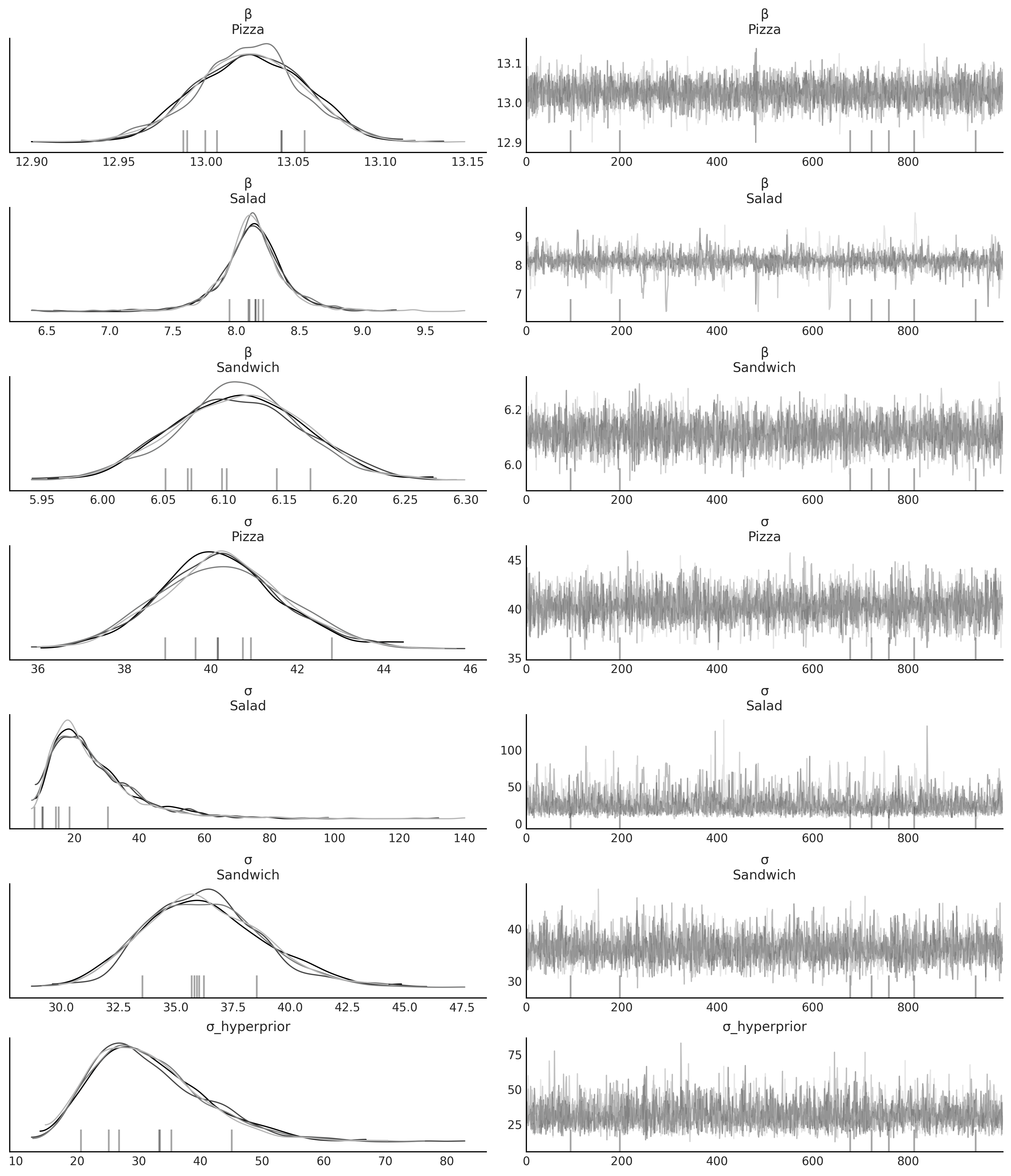
az.summary(inf_data_pooled_sigma_sales, var_names=["β", "σ"])

	mean	sd	hdi_3%	hdi_97%	mcse_mean	mcse_sd	ess_bulk	ess_tail	r_hat
β[0]	13.025	0.030	12.971	13.082	0.000	0.000	7261.0	3250.0	1.0
β[1]	8.128	0.366	7.441	8.776	0.005	0.003	6291.0	3066.0	1.0
β[2]	6.113	0.059	6.003	6.226	0.001	0.001	6336.0	2674.0	1.0
σ	39.257	1.318	36.809	41.689	0.017	0.012	6281.0	2926.0	1.0

Figure 4.20

fig, ax = plt.subplots(figsize=(10, 6))
σ_m = inf_data_sales_pooled.posterior["σ"].mean().values

# Salads

for i in range(3):
    category_mask = (food_category.codes==i)
    μ_m_salads = inf_data_pooled_sigma_sales.posterior["μ"][:,:, category_mask].mean(axis=(0,1))
    ax.plot(sales_df.customers[category_mask], μ_m_salads, c='C4')
    az.plot_hdi(sales_df.customers[category_mask], inf_data_pooled_sigma_sales.posterior_predictive["sales"][:,:, (category_mask)], hdi_prob=.50, ax=ax, fill_kwargs={"alpha": .5})
    #az.plot_hdi(sales_df.customers[category_mask], inf_data_pooled_sigma_sales.posterior_predictive["sales"][:,:, (category_mask)], hdi_prob=.94, ax=ax)


pizza_df.plot(x="customers", y="sales", kind="scatter", ax=ax, c="C1", label="Pizza", marker="^", s=60);
sandwich_df.plot(x="customers", y="sales", kind="scatter", ax=ax,  label="Sandwich", marker="s");
salad_df.plot(x="customers", y="sales", kind="scatter", ax=ax, label="Salad", c="C4");


ax.set_xlabel("Number of Customers")
ax.set_ylabel("Daily Sales Dollars")
ax.set_title("Unpooled Slope Pooled Sigma Regression")
plt.savefig("img/chp04/salad_sales_basic_regression_scatter_sigma_pooled_slope_unpooled.png")

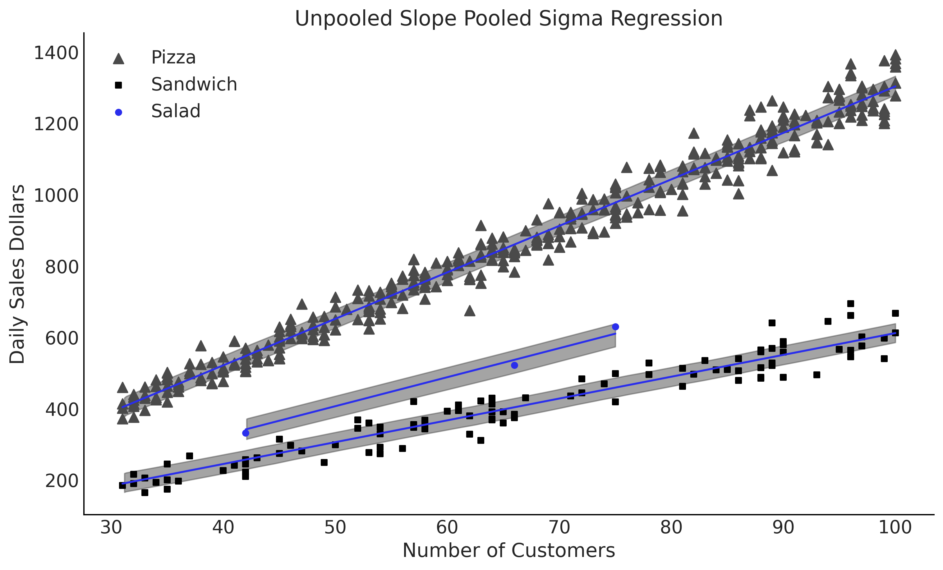
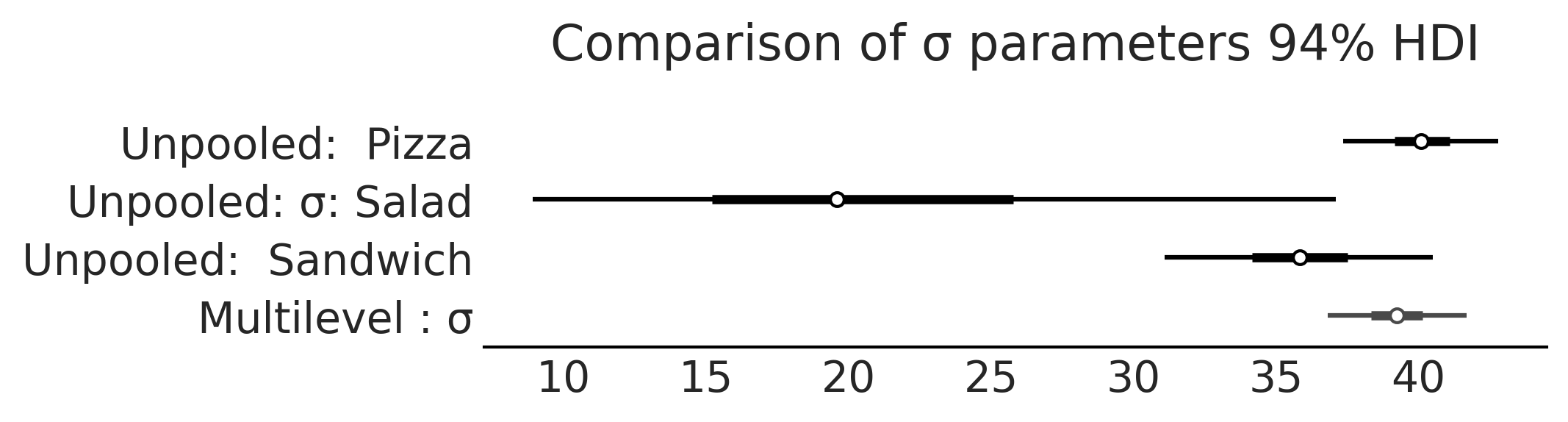
Figure 4.21

axes = az.plot_forest([inf_data_sales_unpooled,
                       inf_data_pooled_sigma_sales
                      ],
                      model_names = ["Unpooled",
                                     "Multilevel "
                                    ],
                      var_names=["σ"], combined=True, figsize=(7, 1.8));
axes[0].set_title("Comparison of σ parameters 94% HDI")

plt.savefig("img/chp04/salad_sales_forestplot_sigma_unpooled_multilevel_comparison.png")

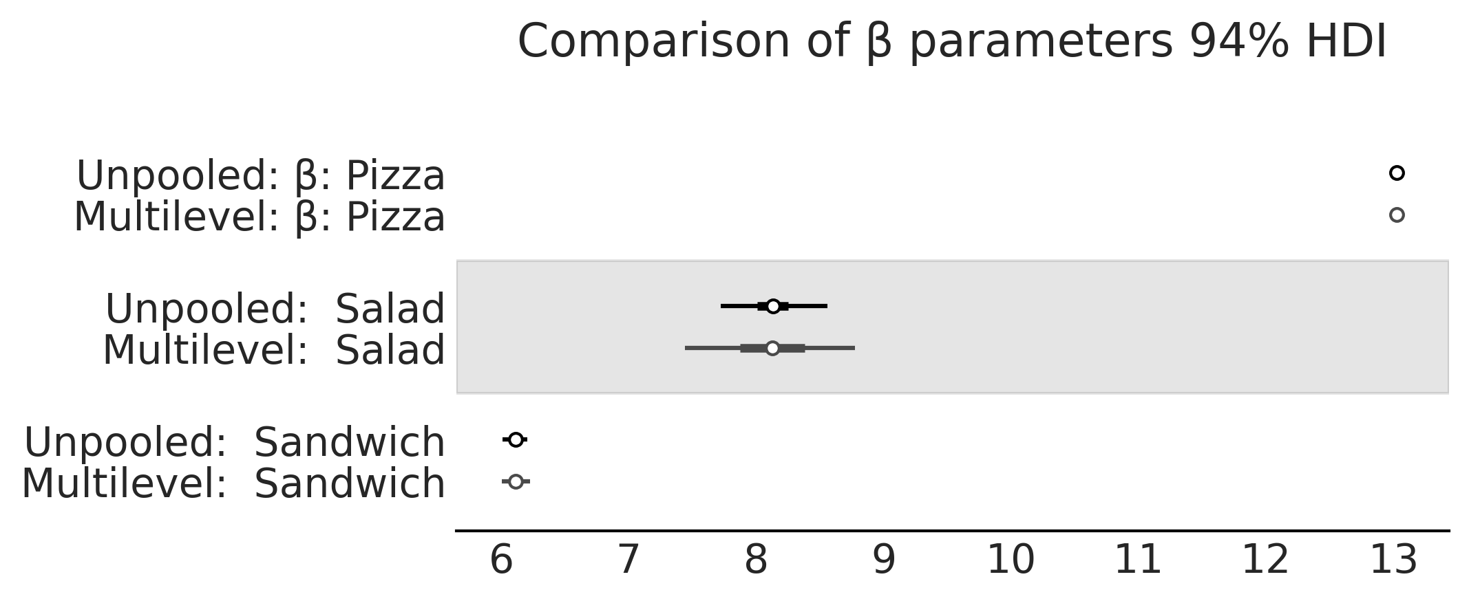
axes = az.plot_forest([inf_data_sales_unpooled,
                       inf_data_pooled_sigma_sales
                      ],
                      model_names = ["Unpooled",
                                     "Multilevel"
                                    ],
                      var_names=["β"], combined=True, figsize=(7, 2.8));
axes[0].set_title("Comparison of β parameters 94% HDI")

Text(0.5, 1.0, 'Comparison of β parameters 94% HDI')

inf_posterior_salads = inf_data_pooled_sigma_sales.posterior.sel(β_dim_0="Salad", μ_dim_0=slice(465, 467))

Hierarchical

Code 4.12

with pm.Model() as model_hierarchical_sales:
    σ_hyperprior = pm.HalfNormal("σ_hyperprior", 20)
    σ = pm.HalfNormal("σ", σ_hyperprior, shape=3)
    
    β = pm.Normal("β", mu=10, sigma=20, shape=3)
    μ = pm.Deterministic("μ", β[food_category.codes] * customers)
    
    sales = pm.Normal("sales", mu=μ, sigma=σ[food_category.codes],
                      observed=sales_observed)
    
    trace_hierarchical_sales = pm.sample(target_accept=.9)
    
    inf_data_hierarchical_sales = az.from_pymc3(
        trace=trace_hierarchical_sales, 
        coords={"β_dim_0":food_category.categories,
                "σ_dim_0":food_category.categories})

/var/folders/7p/srk5qjp563l5f9mrjtp44bh800jqsw/T/ipykernel_8872/2572718925.py:11: FutureWarning: In v4.0, pm.sample will return an `arviz.InferenceData` object instead of a `MultiTrace` by default. You can pass return_inferencedata=True or return_inferencedata=False to be safe and silence this warning.
  trace_hierarchical_sales = pm.sample(target_accept=.9)
Auto-assigning NUTS sampler...
Initializing NUTS using jitter+adapt_diag...
Multiprocess sampling (4 chains in 4 jobs)
NUTS: [β, σ, σ_hyperprior]

100.00% [8000/8000 00:05<00:00 Sampling 4 chains, 7 divergences]

Sampling 4 chains for 1_000 tune and 1_000 draw iterations (4_000 + 4_000 draws total) took 15 seconds.
There were 5 divergences after tuning. Increase `target_accept` or reparameterize.
There were 2 divergences after tuning. Increase `target_accept` or reparameterize.

az.plot_trace(inf_data_hierarchical_sales, compact=False, var_names=["β", "σ", "σ_hyperprior"]);

az.plot_parallel(inf_data_hierarchical_sales, var_names=["σ", "σ_hyperprior"])

<AxesSubplot:>

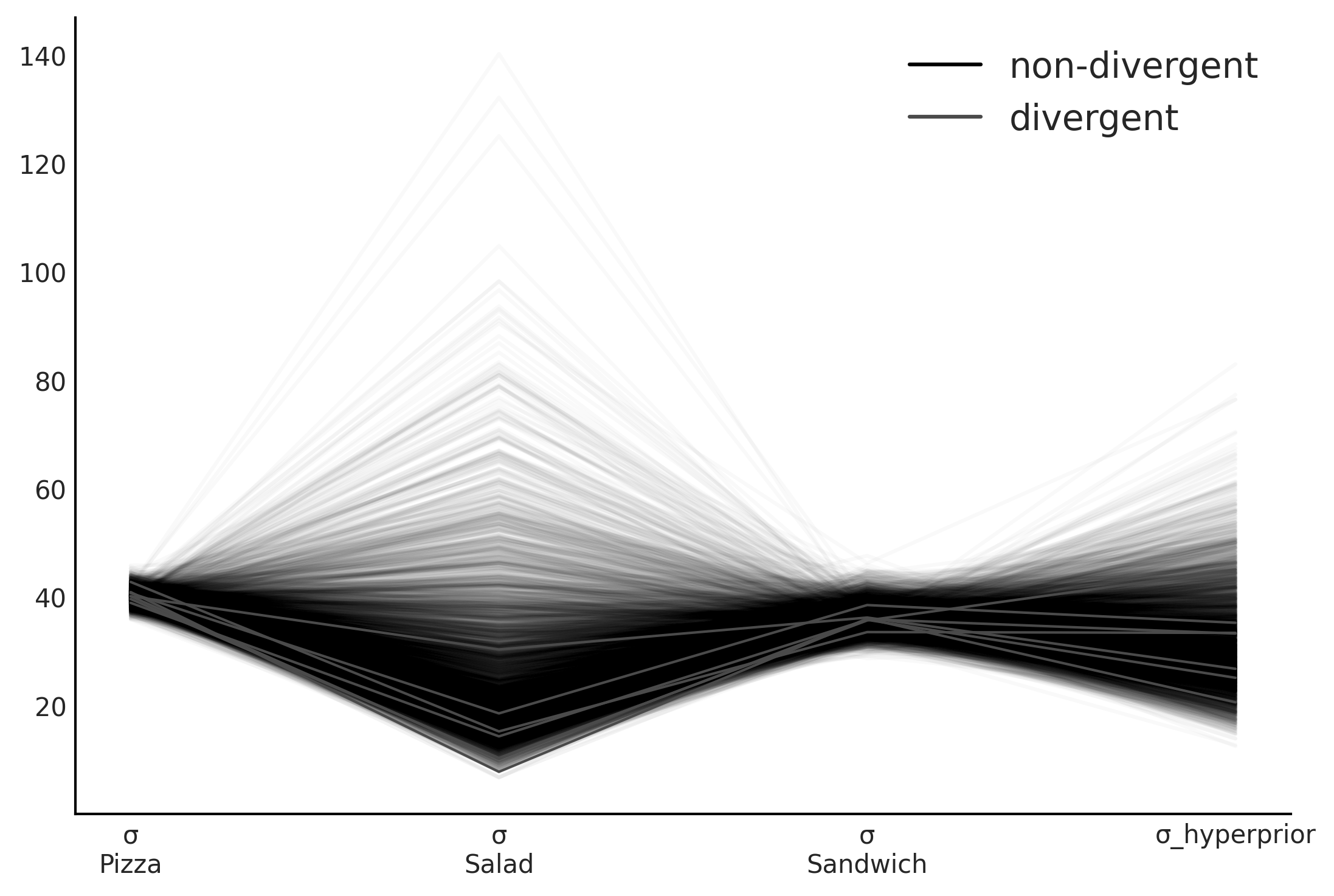
Figure 4.23

hierarchial_sales_diagram = pm.model_to_graphviz(model_hierarchical_sales)
hierarchial_sales_diagram.render("img/chp04/salad_sales_hierarchial_regression_model", format="png", cleanup=True)
hierarchial_sales_diagram

az.summary(inf_data_hierarchical_sales, var_names=["β", "σ"])

	mean	sd	hdi_3%	hdi_97%	mcse_mean	mcse_sd	ess_bulk	ess_tail	r_hat
β[0]	13.025	0.031	12.968	13.082	0.000	0.000	5196.0	2491.0	1.0
β[1]	8.131	0.275	7.613	8.641	0.006	0.004	2558.0	1788.0	1.0
β[2]	6.113	0.053	6.012	6.208	0.001	0.001	4419.0	2689.0	1.0
σ[0]	40.261	1.474	37.489	43.064	0.021	0.015	4979.0	2825.0	1.0
σ[1]	26.007	13.588	7.889	50.398	0.304	0.215	2404.0	2152.0	1.0
σ[2]	36.274	2.604	31.514	41.230	0.038	0.027	4816.0	2676.0	1.0

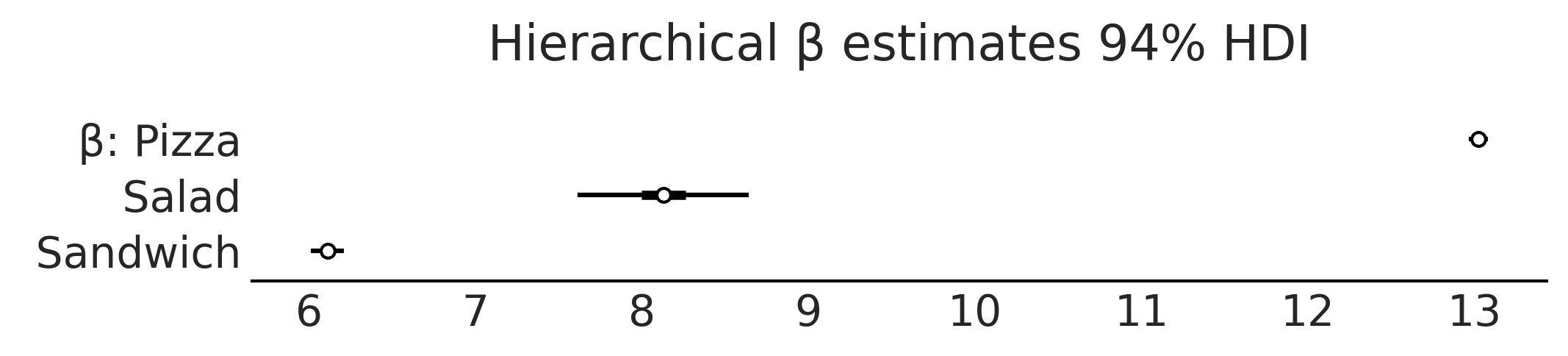
axes = az.plot_forest(inf_data_hierarchical_sales, var_names=["β"], combined=True,  figsize=(7, 1.5))
axes[0].set_title("Hierarchical β estimates 94% HDI")

Text(0.5, 1.0, 'Hierarchical β estimates 94% HDI')

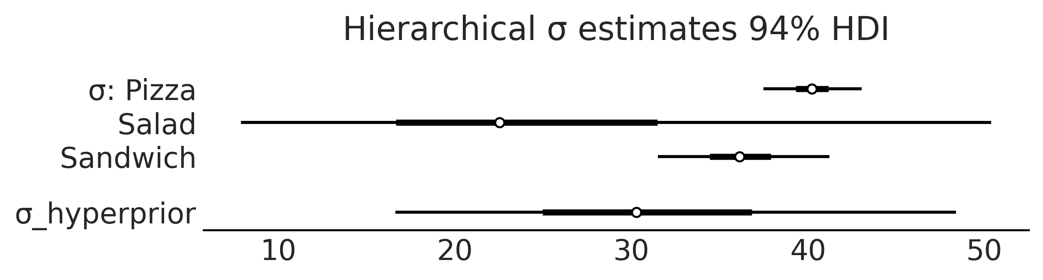
axes = az.plot_forest(inf_data_hierarchical_sales, var_names=["σ", "σ_hyperprior"], combined=True,  figsize=(7, 1.8))
axes[0].set_title("Hierarchical σ estimates 94% HDI")
plt.savefig("img/chp04/salad_sales_forestplot_sigma_hierarchical.png")

print(food_category.categories)

Index(['Pizza', 'Salad', 'Sandwich'], dtype='object')

Table 4.3

az.summary(inf_data_sales_unpooled.posterior["σ"], kind="stats").round(1)

	mean	sd	hdi_3%	hdi_97%
σ[0]	40.1	1.5	37.4	42.8
σ[1]	21.4	8.3	8.9	37.1
σ[2]	35.9	2.5	31.1	40.5

Table 4.4

az.summary(inf_data_hierarchical_sales, var_names=["σ", "σ_hyperprior"], kind="stats").round(1)

	mean	sd	hdi_3%	hdi_97%
σ[0]	40.3	1.5	37.5	43.1
σ[1]	26.0	13.6	7.9	50.4
σ[2]	36.3	2.6	31.5	41.2
σ_hyperprior	31.7	9.1	16.6	48.4

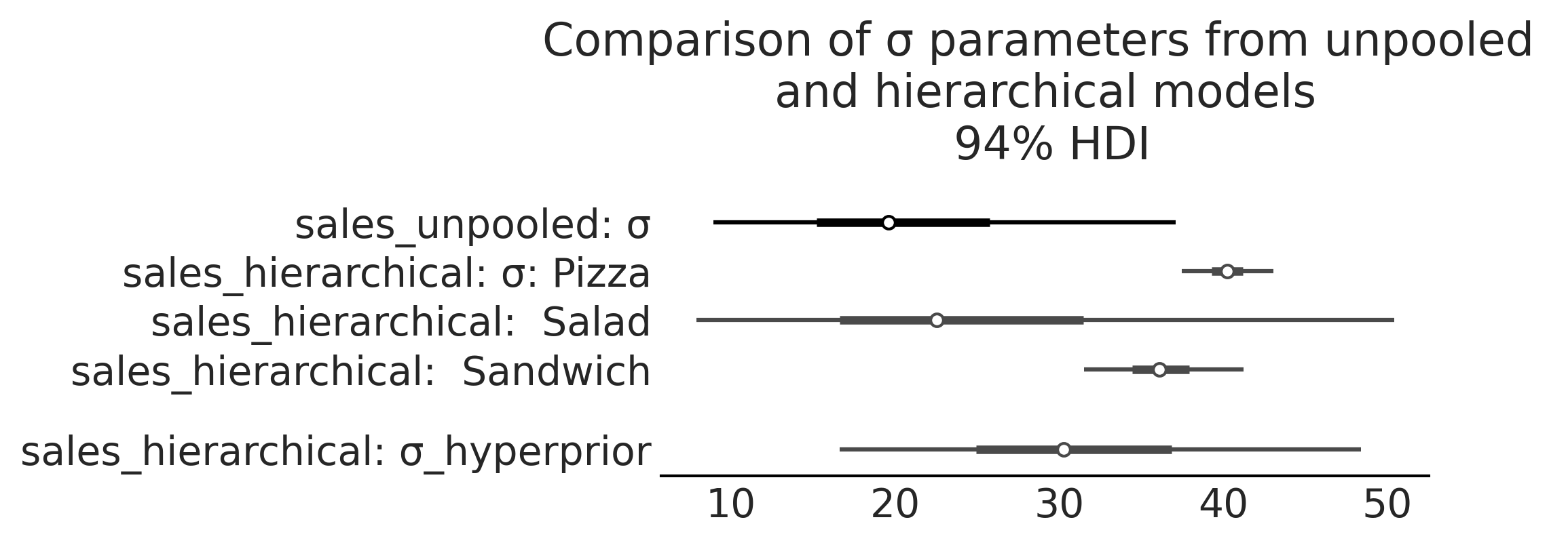
axes = az.plot_forest([inf_data_sales_unpooled.posterior["σ"].isel(σ_dim_0=1),
                       inf_data_hierarchical_sales
                      ],
                      model_names = ["sales_unpooled",
                                     "sales_hierarchical"
                                    ], combined=True, figsize=(7, 2.6),
                     var_names=["σ", "σ_hyperprior"]
                     );
axes[0].set_title("Comparison of σ parameters from unpooled \n and hierarchical models \n 94% HDI")

plt.savefig("img/chp04/salad_sales_forestolot_sigma_unpooled_multilevel_comparison.png")

fig, ax = plt.subplots()
az.plot_kde(inf_data_sales_unpooled.posterior['σ'].isel(σ_dim_0=1), label="Unpooled Salad Sigma", ax=ax)
az.plot_kde(inf_data_hierarchical_sales.posterior["σ"].isel(σ_dim_0=1), label="Hierarchical Salad Sigma", plot_kwargs={"color":"C4"}, ax=ax);

ax.set_title("Comparison of Hierarchical versus Unpooled Variance")

Text(0.5, 1.0, 'Comparison of Hierarchical versus Unpooled Variance')

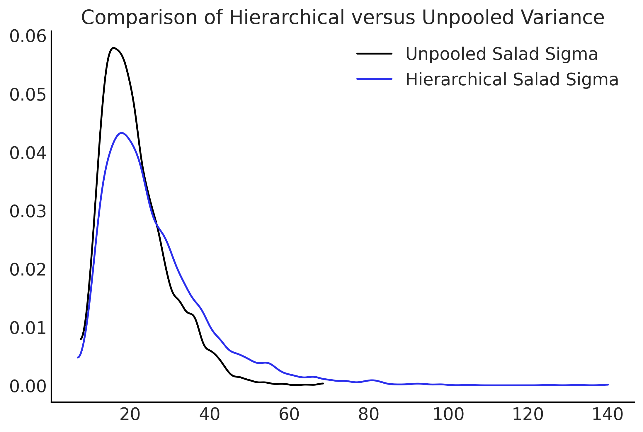
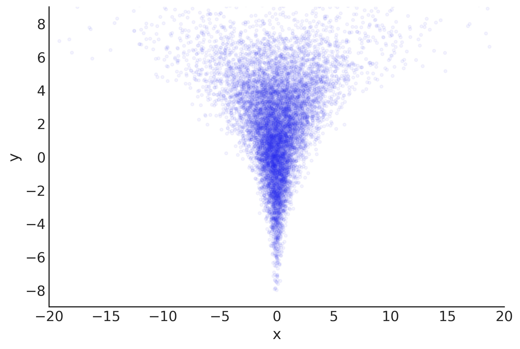
Figure 4.25

nsample = 10000
nd=1
yr = stats.norm.rvs(loc=2., scale=3., size=nsample)
xnr = stats.norm.rvs(loc=0., scale=np.exp(yr/4), size=(nd, nsample))

fig, ax = plt.subplots()
ax.scatter(xnr[0], yr, marker='.', alpha=.05, color="C4")
ax.set_xlim(-20, 20)
ax.set_ylim(-9, 9)
ax.set_xlabel('x')
ax.set_ylabel('y')

Text(0, 0.5, 'y')

def salad_generator(hyperprior_beta_mean=5, hyperprior_beta_sigma=.2, sigma=50, days_per_location=[6, 4, 15, 10, 3, 5], sigma_per_location=[50,10,20,80,30,20]):
    """Generate noisy salad data"""
    beta_hyperprior = stats.norm(hyperprior_beta_mean, hyperprior_beta_sigma)
    
    # Generate demands days per restaurant
    df = pd.DataFrame()
    for i, days in enumerate(days_per_location):
        np.random.seed(0)

        num_customers = stats.randint(30, 100).rvs(days)
        sales_location = beta_hyperprior.rvs()*num_customers + stats.norm(0, sigma_per_location[i]).rvs(num_customers.shape)

        location_df = pd.DataFrame({"customers":num_customers, "sales":sales_location})
        location_df["location"] = i
        location_df.sort_values(by="customers", ascending=True)
        df = pd.concat([df, location_df])
        
    df.reset_index(inplace=True, drop=True)
    return df
hierarchical_salad_df = salad_generator()

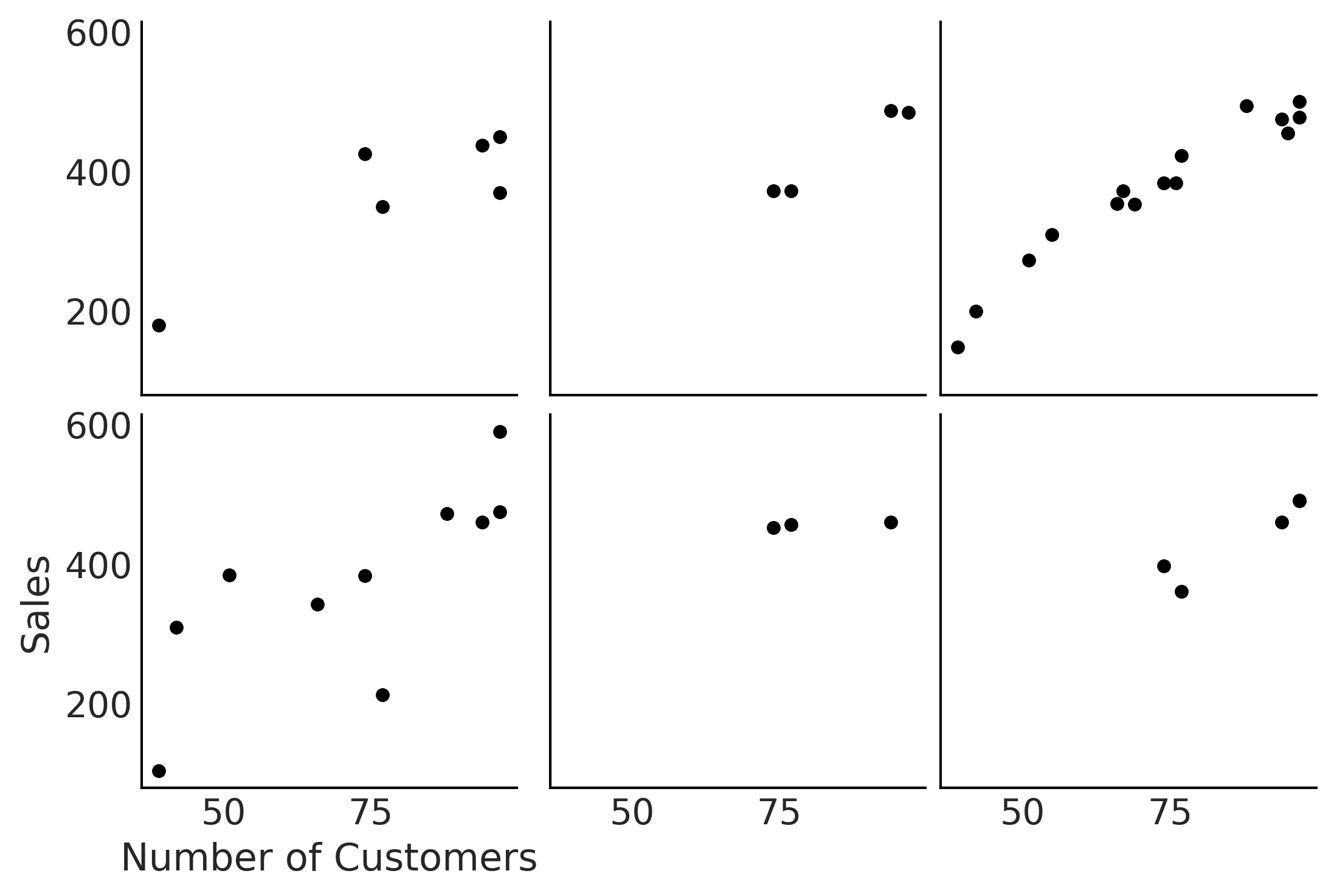
Figure 4.26

fig, axes, = plt.subplots(2,3, sharex=True, sharey=True)

for i, ax in enumerate(axes.ravel()):
    location_filter = (hierarchical_salad_df["location"] == i)
    hierarchical_salad_df[location_filter].plot(kind="scatter", x="customers", y="sales", ax=ax)
    ax.set_xlabel("")
    ax.set_ylabel("")

    
axes[1,0].set_xlabel("Number of Customers")
axes[1,0].set_ylabel("Sales");
plt.savefig("img/chp04/multiple_salad_sales_scatter.png")

Code 4.13

import tensorflow as tf
import tensorflow_probability as tfp

tfd = tfp.distributions
root = tfd.JointDistributionCoroutine.Root

run_mcmc = tf.function(
    tfp.experimental.mcmc.windowed_adaptive_nuts,
    autograph=False, jit_compile=True)

def gen_hierarchical_salad_sales(input_df, beta_prior_fn, dtype=tf.float32):
    customers = tf.constant(
        hierarchical_salad_df["customers"].values, dtype=dtype)
    location_category = hierarchical_salad_df["location"].values
    sales = tf.constant(hierarchical_salad_df["sales"].values, dtype=dtype)

    @tfd.JointDistributionCoroutine
    def model_hierarchical_salad_sales():
        β_μ_hyperprior = yield root(tfd.Normal(0, 10, name="beta_mu"))
        β_σ_hyperprior = yield root(tfd.HalfNormal(.1, name="beta_sigma"))
        β = yield from beta_prior_fn(β_μ_hyperprior, β_σ_hyperprior)

        σ_hyperprior = yield root(tfd.HalfNormal(30, name="sigma_prior"))
        σ = yield tfd.Sample(tfd.HalfNormal(σ_hyperprior), 6, name="sigma")

        loc = tf.gather(β, location_category, axis=-1) * customers
        scale = tf.gather(σ, location_category, axis=-1)
        sales = yield tfd.Independent(tfd.Normal(loc, scale),
                                      reinterpreted_batch_ndims=1,
                                      name="sales")

    return model_hierarchical_salad_sales, sales

Code 4.14 and 4.15

def centered_beta_prior_fn(hyper_mu, hyper_sigma):
    β = yield tfd.Sample(tfd.Normal(hyper_mu, hyper_sigma), 6, name="beta")
    return β

# hierarchical_salad_df is the generated dataset as pandas.DataFrame
centered_model, observed = gen_hierarchical_salad_sales(
    hierarchical_salad_df, centered_beta_prior_fn)

mcmc_samples_centered, sampler_stats_centered = run_mcmc(
    1000, centered_model, n_chains=4, num_adaptation_steps=1000,
    sales=observed)

divergent_per_chain = np.sum(sampler_stats_centered['diverging'], axis=0)
print(f"""There were {divergent_per_chain} divergences after tuning per chain.""")

WARNING:tensorflow:From /opt/miniconda3/envs/bmcp/lib/python3.9/site-packages/tensorflow_probability/python/distributions/distribution.py:342: calling MultivariateNormalDiag.__init__ (from tensorflow_probability.python.distributions.mvn_diag) with scale_identity_multiplier is deprecated and will be removed after 2020-01-01.
Instructions for updating:
`scale_identity_multiplier` is deprecated; please combine it into `scale_diag` directly instead.

2021-11-19 16:49:41.809766: W tensorflow/compiler/tf2xla/kernels/random_ops.cc:102] Warning: Using tf.random.uniform with XLA compilation will ignore seeds; consider using tf.random.stateless_uniform instead if reproducible behavior is desired. sanitize_seed/seed
2021-11-19 16:49:41.952731: W tensorflow/compiler/tf2xla/kernels/assert_op.cc:38] Ignoring Assert operator mcmc_retry_init/assert_equal_1/Assert/AssertGuard/Assert

There were [ 24 112 194  44] divergences after tuning per chain.

idata_centered_model = az.from_dict(
    posterior={
        k:np.swapaxes(v, 1, 0)
        for k, v in mcmc_samples_centered._asdict().items()},
    sample_stats={
        k:np.swapaxes(sampler_stats_centered[k], 1, 0)
        for k in ["target_log_prob", "diverging", "accept_ratio", "n_steps"]}
)

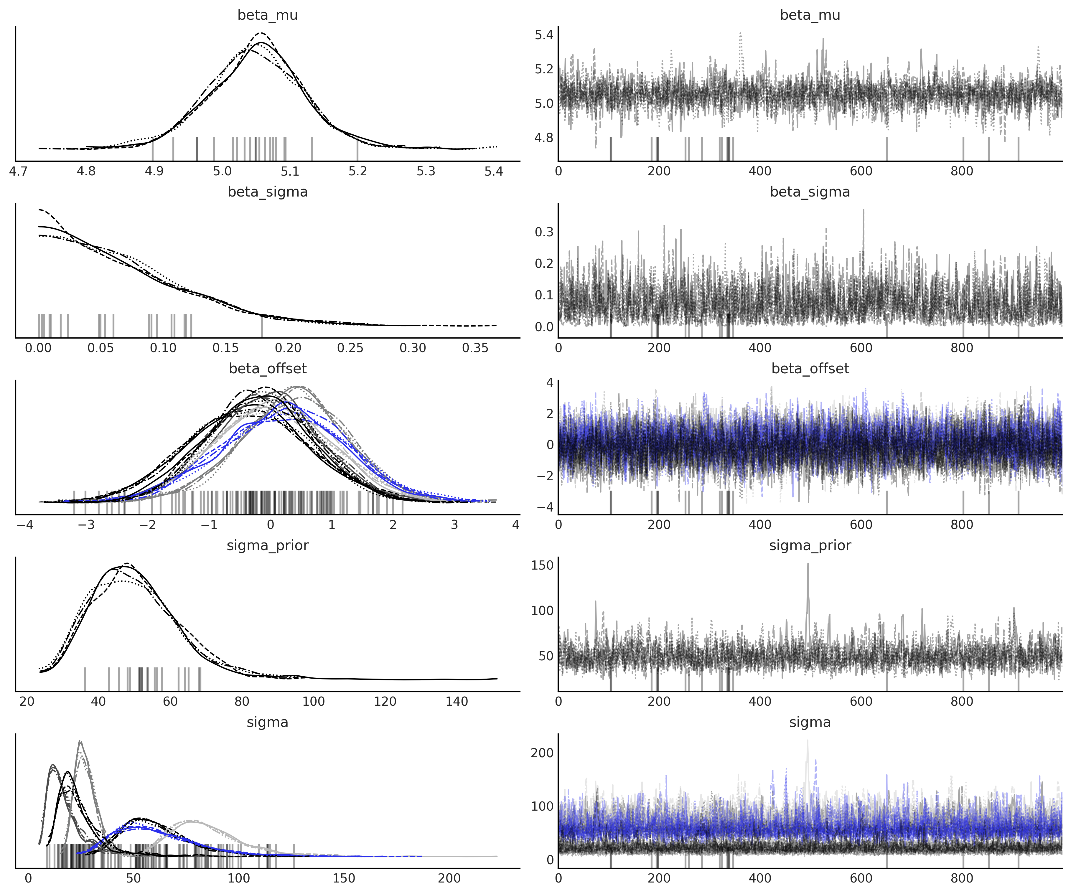
az.plot_trace(idata_centered_model, compact=True);

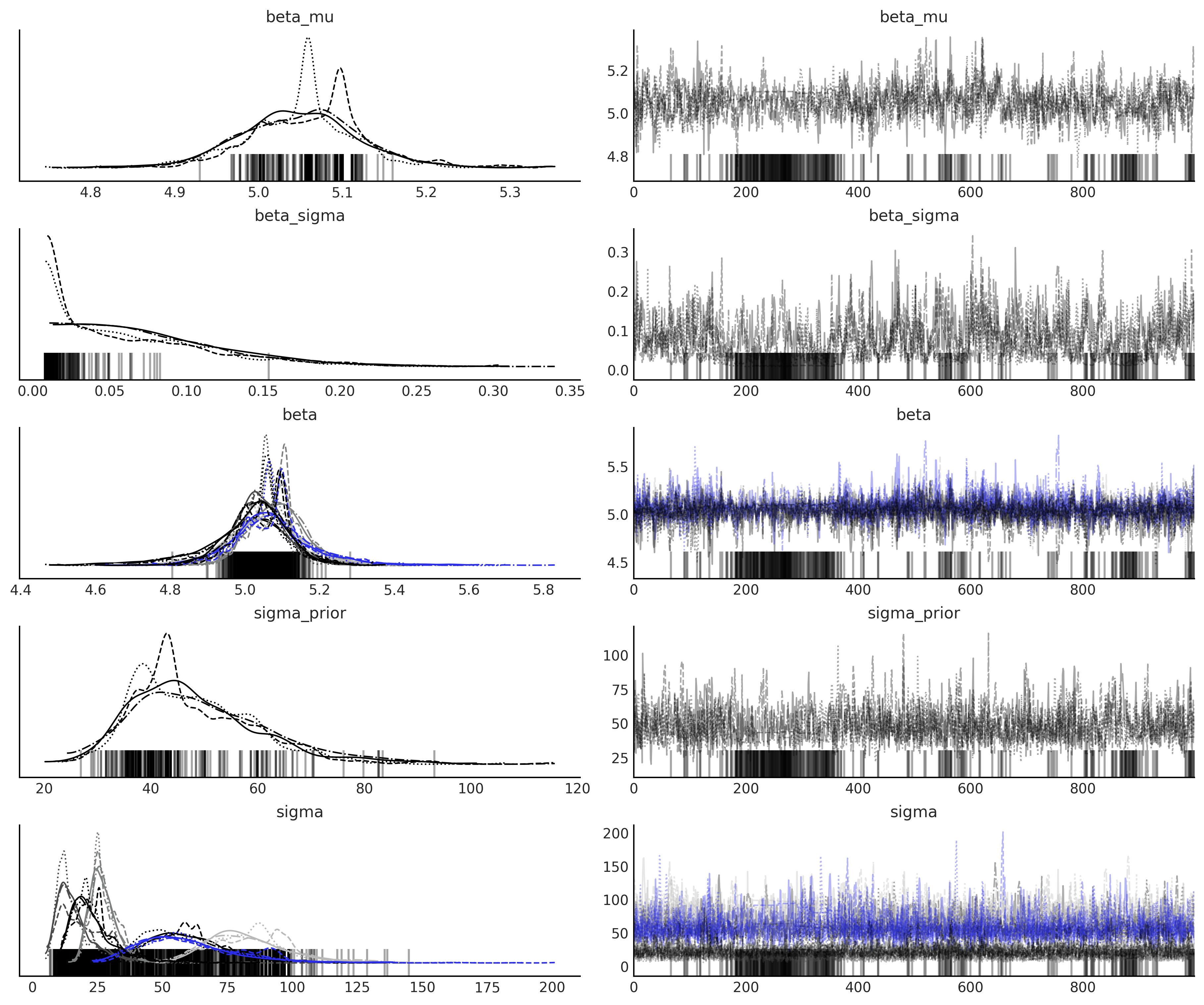
az.summary(idata_centered_model)

	mean	sd	hdi_3%	hdi_97%	mcse_mean	mcse_sd	ess_bulk	ess_tail	r_hat
beta_mu	5.053	0.071	4.911	5.179	0.003	0.002	451.0	1462.0	1.02
beta_sigma	0.072	0.053	0.008	0.167	0.004	0.003	90.0	54.0	1.05
beta[0]	5.012	0.118	4.759	5.217	0.004	0.003	653.0	1563.0	1.02
beta[1]	5.042	0.071	4.908	5.174	0.003	0.002	591.0	1775.0	1.02
beta[2]	5.087	0.073	4.949	5.225	0.003	0.002	713.0	1453.0	1.01
beta[3]	5.057	0.100	4.865	5.261	0.003	0.002	855.0	1370.0	1.01
beta[4]	5.076	0.112	4.864	5.289	0.003	0.002	1059.0	1600.0	1.01
beta[5]	5.041	0.077	4.878	5.176	0.002	0.002	724.0	1966.0	1.01
sigma_prior	48.410	12.377	27.661	71.280	0.427	0.302	905.0	1645.0	1.01
sigma[0]	59.925	16.018	35.037	90.595	0.715	0.506	379.0	340.0	1.02
sigma[1]	17.692	9.324	6.065	32.821	0.774	0.548	203.0	1209.0	1.03
sigma[2]	27.447	5.538	18.332	37.794	0.196	0.146	1050.0	761.0	1.00
sigma[3]	83.552	16.075	54.561	111.829	0.480	0.340	794.0	1345.0	1.01
sigma[4]	60.412	19.803	29.284	93.902	1.080	0.765	375.0	1595.0	1.01
sigma[5]	23.581	9.324	9.895	40.715	0.301	0.229	1089.0	932.0	1.01

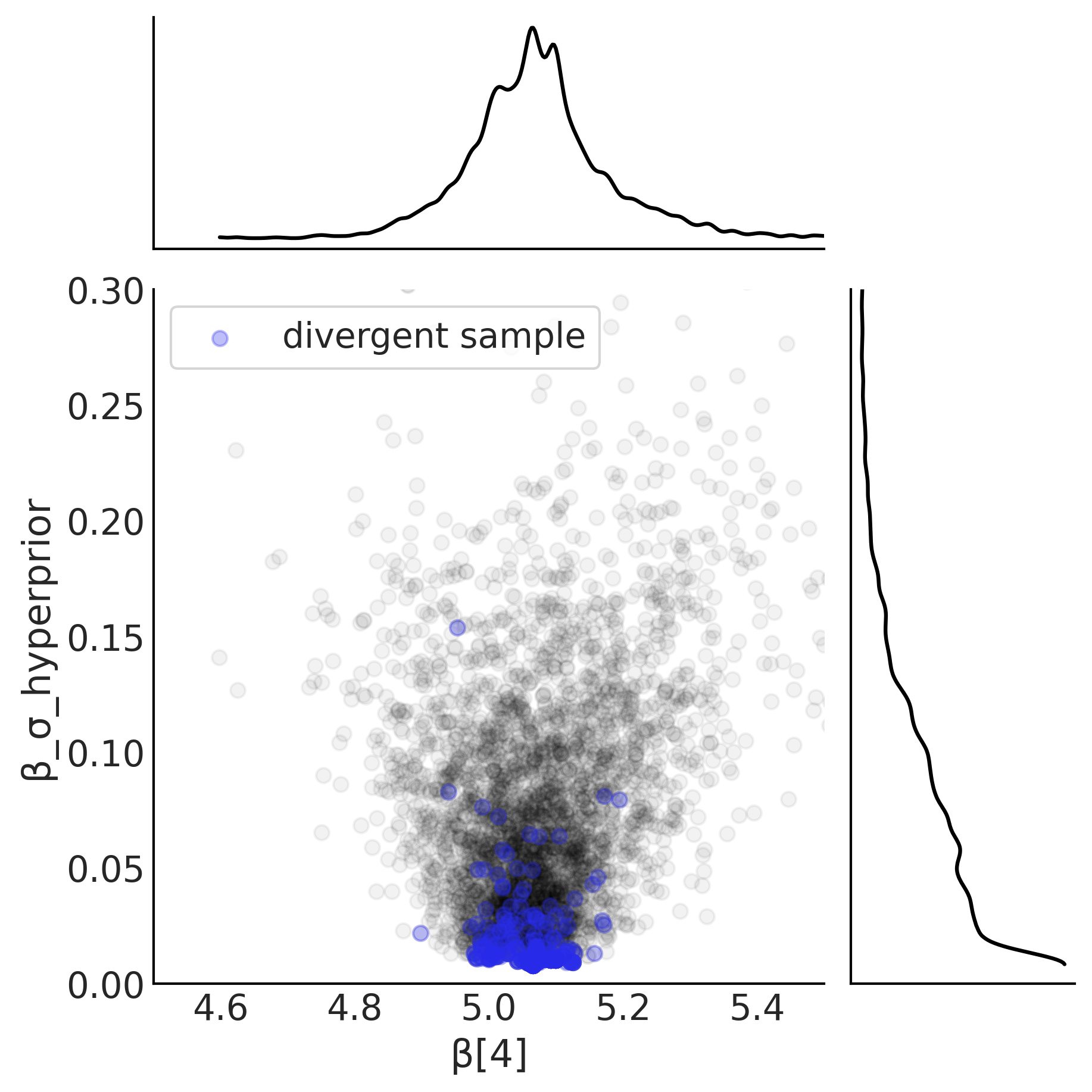
Figure 4.27

slope = mcmc_samples_centered.beta[..., 4].numpy().flatten()
sigma = mcmc_samples_centered.beta_sigma.numpy().flatten()
divergences = sampler_stats_centered['diverging'].numpy().flatten()

axes = az.plot_joint({"β[4]": slope, "β_σ_hyperprior": sigma},
                     joint_kwargs={"alpha": .05}, figsize=(6, 6))
axes[0].scatter(slope[divergences], sigma[divergences], c="C4", alpha=.3, label='divergent sample')
axes[0].legend(frameon=True)
axes[0].set_ylim(0, .3)
axes[0].set_xlim(4.5, 5.5)

plt.savefig("img/chp04/Neals_Funnel_Salad_Centered.png")

/opt/miniconda3/envs/bmcp/lib/python3.9/site-packages/arviz/plots/jointplot.py:144: UserWarning: plot_joint will be deprecated. Please use plot_pair instead.
  warnings.warn("plot_joint will be deprecated. Please use plot_pair instead.")

Code 4.16

def non_centered_beta_prior_fn(hyper_mu, hyper_sigma):
    β_offset = yield root(tfd.Sample(tfd.Normal(0, 1), 6, name="beta_offset"))
    return β_offset * hyper_sigma[..., None] + hyper_mu[..., None]

# hierarchical_salad_df is the generated dataset as pandas.DataFrame
non_centered_model, observed = gen_hierarchical_salad_sales(
    hierarchical_salad_df, non_centered_beta_prior_fn)

mcmc_samples_noncentered, sampler_stats_noncentered = run_mcmc(
    1000, non_centered_model, n_chains=4, num_adaptation_steps=1000,
    sales=observed)

divergent_per_chain = np.sum(sampler_stats_noncentered['diverging'], axis=0)
print(f"""There were {divergent_per_chain} divergences after tuning per chain.""")

2021-11-19 16:50:17.643939: W tensorflow/compiler/tf2xla/kernels/assert_op.cc:38] Ignoring Assert operator mcmc_retry_init/assert_equal_1/Assert/AssertGuard/Assert

There were [ 0  0 20  0] divergences after tuning per chain.

idata_non_centered_model = az.from_dict(
    posterior={
        k:np.swapaxes(v, 1, 0)
        for k, v in mcmc_samples_noncentered._asdict().items()},
    sample_stats={
        k:np.swapaxes(sampler_stats_noncentered[k], 1, 0)
        for k in ["target_log_prob", "diverging", "accept_ratio", "n_steps"]}
)

az.plot_trace(idata_non_centered_model, compact=True);

az.summary(idata_non_centered_model)

	mean	sd	hdi_3%	hdi_97%	mcse_mean	mcse_sd	ess_bulk	ess_tail	r_hat
beta_mu	5.050	0.073	4.914	5.188	0.002	0.001	2006.0	2092.0	1.0
beta_sigma	0.069	0.054	0.000	0.163	0.001	0.001	1384.0	1262.0	1.0
beta_offset[0]	-0.366	0.996	-2.141	1.592	0.018	0.015	3061.0	2485.0	1.0
beta_offset[1]	-0.096	0.885	-1.761	1.557	0.018	0.014	2556.0	2648.0	1.0
beta_offset[2]	0.392	0.890	-1.339	2.047	0.018	0.013	2457.0	2927.0	1.0
beta_offset[3]	0.040	0.972	-1.685	1.930	0.017	0.016	3099.0	2785.0	1.0
beta_offset[4]	0.230	1.038	-1.738	2.169	0.019	0.017	2940.0	2233.0	1.0
beta_offset[5]	-0.154	0.872	-1.794	1.466	0.017	0.013	2508.0	2880.0	1.0
sigma_prior	50.026	12.585	28.433	72.742	0.320	0.242	1842.0	1525.0	1.0
sigma[0]	60.975	16.688	33.831	93.832	0.400	0.307	2291.0	1523.0	1.0
sigma[1]	18.473	11.477	6.049	37.322	0.511	0.402	1086.0	601.0	1.0
sigma[2]	27.445	5.453	18.557	38.042	0.114	0.086	2785.0	1787.0	1.0
sigma[3]	83.830	17.153	55.301	114.967	0.418	0.330	2335.0	1584.0	1.0
sigma[4]	60.699	20.419	29.070	98.661	0.470	0.369	2558.0	1826.0	1.0
sigma[5]	24.146	10.760	10.322	42.645	0.400	0.322	1400.0	821.0	1.0

Figure 4.28

noncentered_beta = (mcmc_samples_noncentered.beta_mu[..., None]
        + mcmc_samples_noncentered.beta_offset * mcmc_samples_noncentered.beta_sigma[..., None])
slope = noncentered_beta[..., 4].numpy().flatten()
sigma = mcmc_samples_noncentered.beta_sigma.numpy().flatten()
divergences = sampler_stats_noncentered['diverging'].numpy().flatten()

axes = az.plot_joint({"β[4]": slope, "β_σ_hyperprior": sigma},
                     joint_kwargs={"alpha": .05}, figsize=(6, 6))
axes[0].scatter(slope[divergences], sigma[divergences], c="C4", alpha=.3, label='divergent sample')
axes[0].legend(frameon=True)
axes[0].set_ylim(0, .3)
axes[0].set_xlim(4.5, 5.5)

plt.savefig("img/chp04/Neals_Funnel_Salad_NonCentered.png")

/opt/miniconda3/envs/bmcp/lib/python3.9/site-packages/arviz/plots/jointplot.py:144: UserWarning: plot_joint will be deprecated. Please use plot_pair instead.
  warnings.warn("plot_joint will be deprecated. Please use plot_pair instead.")

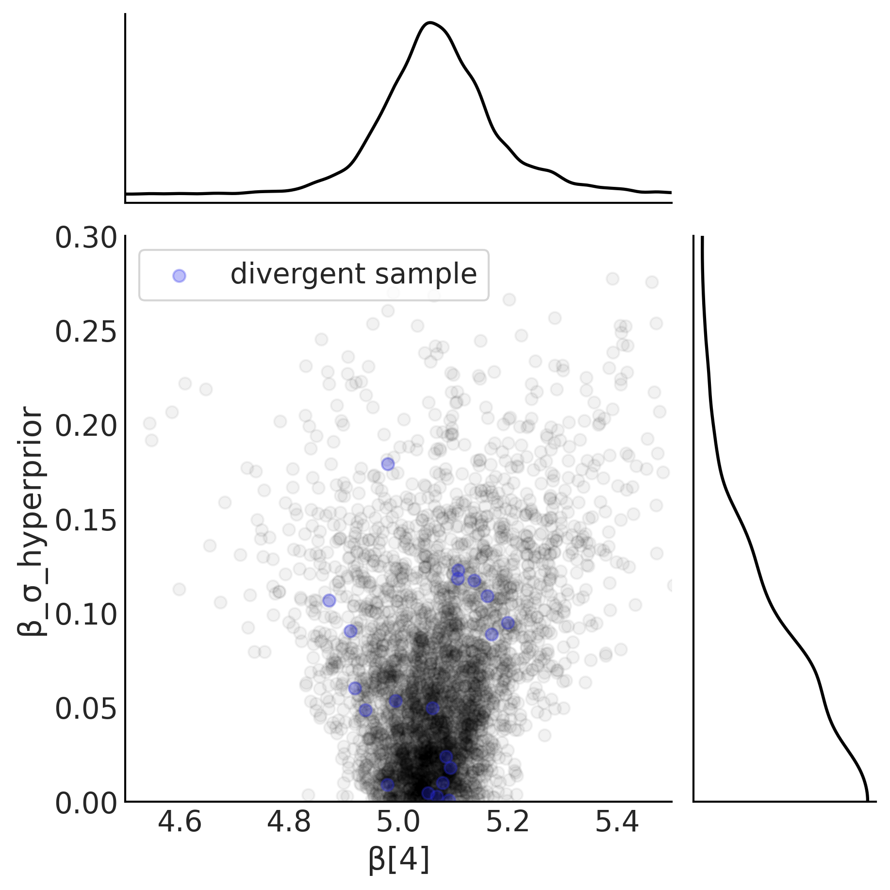
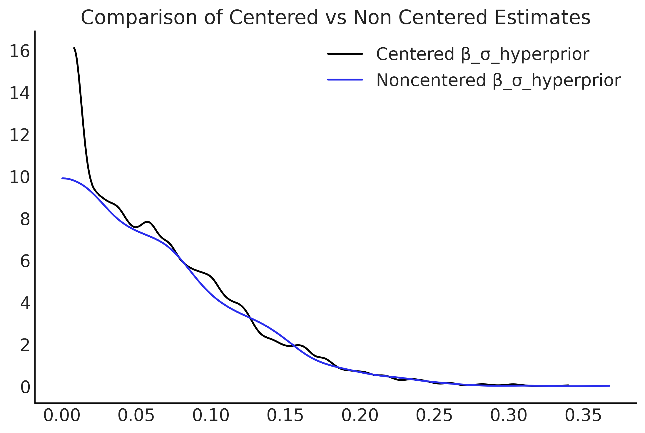
Figure 4.29

centered_β_sigma = mcmc_samples_centered.beta_sigma.numpy()
noncentered_β_sigma = mcmc_samples_noncentered.beta_sigma.numpy()

fig, ax = plt.subplots()
az.plot_kde(centered_β_sigma, label="Centered β_σ_hyperprior", ax=ax)
az.plot_kde(noncentered_β_sigma, label="Noncentered β_σ_hyperprior", plot_kwargs={"color":"C4"}, ax=ax);

ax.set_title("Comparison of Centered vs Non Centered Estimates");
plt.savefig("img/chp04/Salad_Sales_Hierarchical_Comparison.png")

Code 4.17

out_of_sample_customers = 50.

@tfd.JointDistributionCoroutine
def out_of_sample_prediction_model():
    model = yield root(non_centered_model)
    β = model.beta_offset * model.beta_sigma[..., None] + model.beta_mu[..., None]
    
    β_group = yield tfd.Normal(
        model.beta_mu, model.beta_sigma, name="group_beta_prediction")
    group_level_prediction = yield tfd.Normal(
        β_group * out_of_sample_customers,
        model.sigma_prior,
        name="group_level_prediction")
    for l in [2, 4]:
        yield tfd.Normal(
            tf.gather(β, l, axis=-1) * out_of_sample_customers,
            tf.gather(model.sigma, l, axis=-1),
            name=f"location_{l}_prediction")

amended_posterior = tf.nest.pack_sequence_as(
    non_centered_model.sample(),
    list(mcmc_samples_noncentered) + [observed],
)
ppc = out_of_sample_prediction_model.sample(var0=amended_posterior)

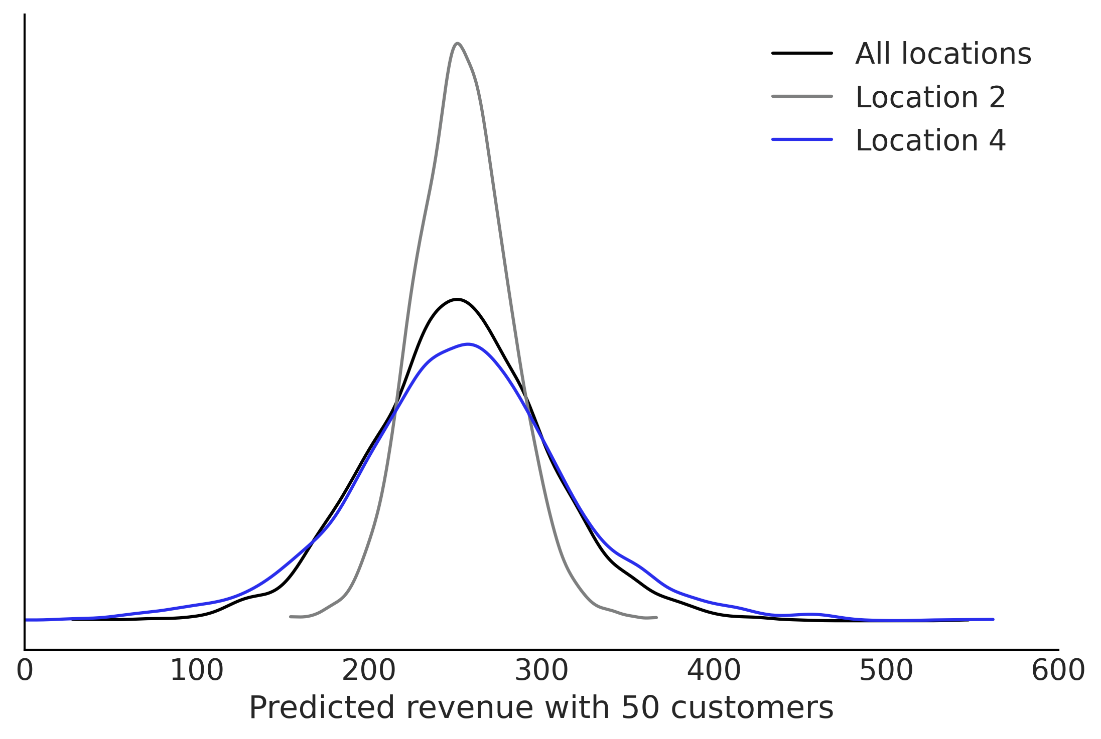
fig, ax = plt.subplots()

az.plot_kde(ppc.group_level_prediction, plot_kwargs={"color":"C0"}, ax=ax, label="All locations")
az.plot_kde(ppc.location_2_prediction, plot_kwargs={"color":"C2"}, ax=ax, label="Location 2")
az.plot_kde(ppc.location_4_prediction, plot_kwargs={"color":"C4"}, ax=ax, label="Location 4")

ax.set_xlabel("Predicted revenue with 50 customers")
ax.set_xlim([0,600])

ax.set_yticks([])

plt.savefig("img/chp04/Salad_Sales_Hierarchical_Predictions.png")

Code 4.18

out_of_sample_customers2 = np.arange(50, 90)

@tfd.JointDistributionCoroutine
def out_of_sample_prediction_model2():
    model = yield root(non_centered_model)
    
    β_new_loc = yield tfd.Normal(
        model.beta_mu, model.beta_sigma, name="beta_new_loc")
    σ_new_loc = yield tfd.HalfNormal(model.sigma_prior, name="sigma_new_loc")
    group_level_prediction = yield tfd.Normal(
        β_new_loc[..., None] * out_of_sample_customers2,
        σ_new_loc[..., None],
        name="new_location_prediction")

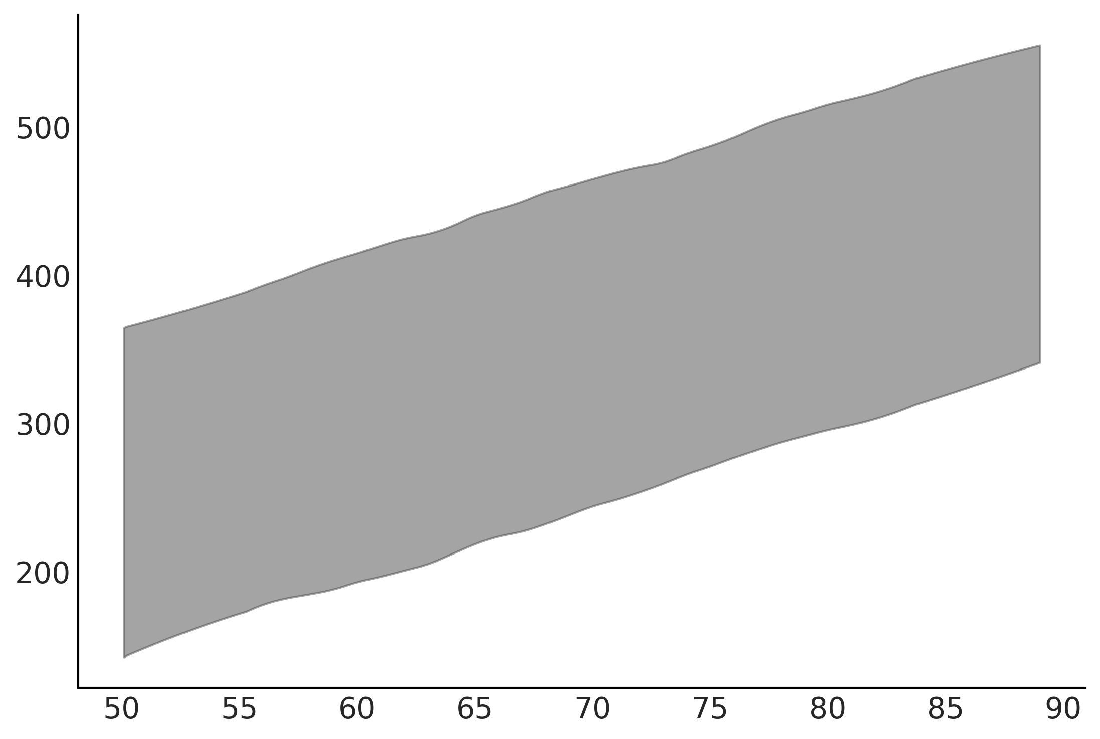
ppc = out_of_sample_prediction_model2.sample(var0=amended_posterior)

az.plot_hdi(out_of_sample_customers2, ppc.new_location_prediction, hdi_prob=.95)

/opt/miniconda3/envs/bmcp/lib/python3.9/site-packages/arviz/data/base.py:169: UserWarning: More chains (1000) than draws (4). Passed array should have shape (chains, draws, *shape)
  warnings.warn(

<AxesSubplot:>