6. Time Series#
“It is difficult to make predictions, especially about the future”. This is true when dutch politician Karl Kristian Steincke allegedly said this sometime in the 1940s [1], and it is still true today especially if you are working on time series and forecasting problems. There are many applications of time series analysis, from making predictions with forecasting, to understanding what were the underlying latent factors in the historical trend. In this chapter we will discuss some Bayesian approaches to this problem. We will start by considering time series modeling as a regression problem, with the design matrices parsed from the timestamp information. We will then explore the approaches to model temporal correlation using autoregressive components. These models extend into a wider (more general) class of State Space Model and Bayesian Structural Time Series model (BSTS), and we will introduce a specialized inference method in the linear Gaussian cases: Kalman Filter. The remainder of the chapter will give a brief summary of model comparison as well as considerations to be made when choosing prior distributions for time series models.
6.1. An Overview of Time Series Problems#
In many real life applications we observe data sequentially in time, generating timestamps along the way each time we make an observation. In addition to the observation itself, the timestamp information can be quite informative when:
There is a temporal trend, for example, regional population, global GDP, annual CO₂ emissions in the US. Usually this is an overall pattern which we intuitively label as “growth” or “decline”.
There is some recurrent pattern correlated to time, called seasonality [2]. For example, changes in monthly temperature (higher in the summer and lower in the winter), monthly rainfall amounts (in many regions of the world this is lower in winter and higher during summer), daily coffee consumption in a given office building (higher in the weekdays and lower in the weekends), hourly number of bike rentals(higher in the day than during the night), like we saw in Chapter 5.
The current data point informs the next data point in some way. In other words where noise or residuals are correlated [3]. For example, the daily number of cases resolved at a help desk, stock price, hourly temperature, hourly rainfall amounts.
It is thus quite natural and useful to consider the decomposition of a time series into:
Most of the classical time series models are based on this decomposition. In this chapter, we will discuss modeling approaches on time series that display some level of temporal trend and seasonality, and explore methods to capture these regular patterns, as well as the less-regular patterns (e.g., residuals correlated in time).
6.2. Time Series Analysis as a Regression Problem#
We will start with modeling a time series with a linear regression model on a widely used demo data set that appears in many tutorials (e.g., PyMC3, TensorFlow Probability) and it was used as an example in the Gaussian Processes for Machine Learning book by Rasmussen and Williams [52]. Atmospheric CO₂ measurements have been taken regularly at the Mauna Loa observatory in Hawaii since the late 1950s at hourly intervals. In many examples the observations are aggregated into monthly average as shown in Fig. 6.1. We load the data into Python with Code Block load_co2_data, and also split the data set into training and testing set. We will fit the model using the training set only, and evaluate the forecast against the testing set.
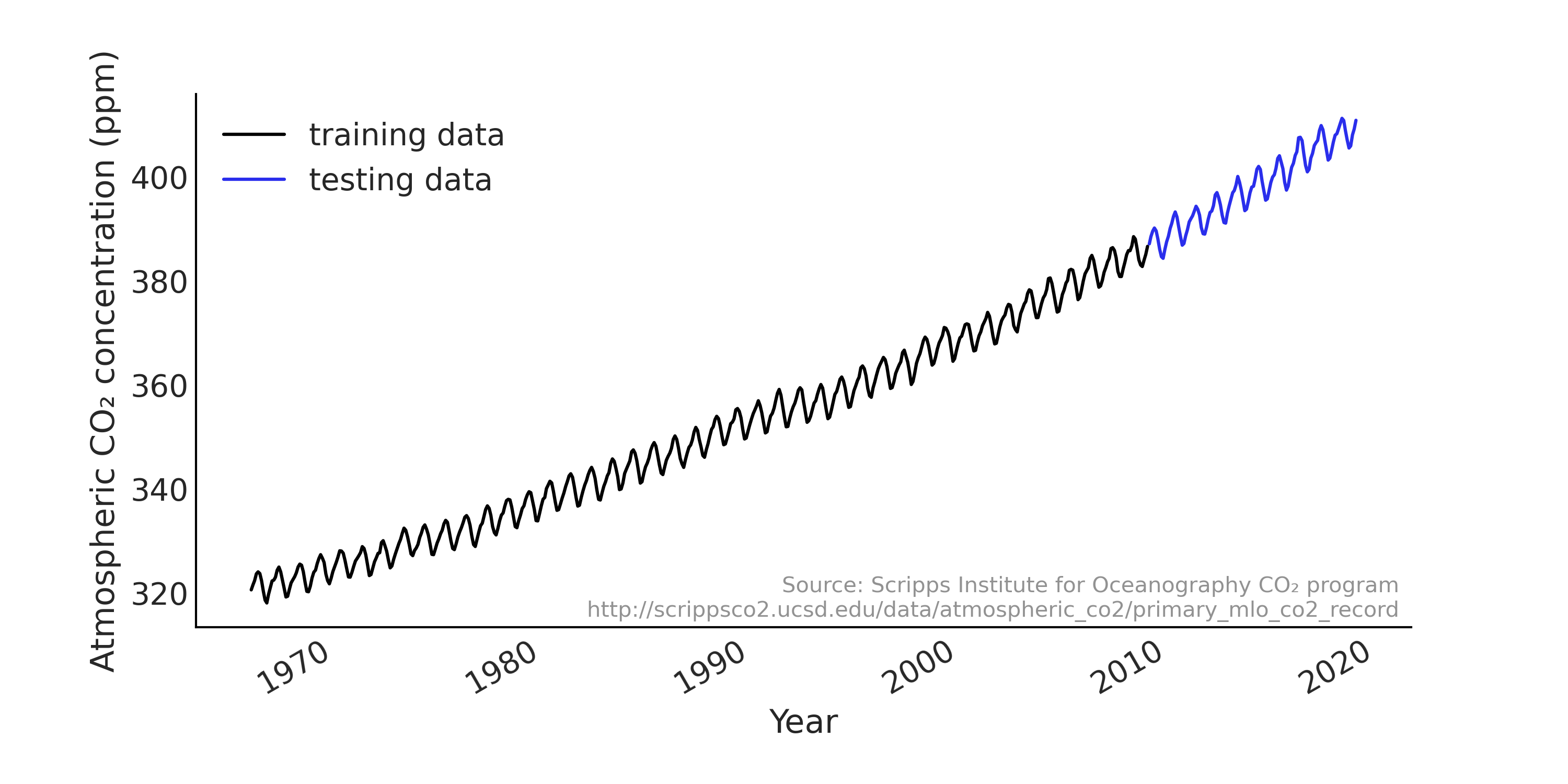
Fig. 6.1 Monthly CO₂ measurements in Mauna Loa from 1966 January to 2019 February, split into training (shown in black) and testing (shown in blue) set. We can see a strong upward trend and seasonality pattern in the data.#
co2_by_month = pd.read_csv("../data/monthly_mauna_loa_co2.csv")
co2_by_month["date_month"] = pd.to_datetime(co2_by_month["date_month"])
co2_by_month["CO2"] = co2_by_month["CO2"].astype(np.float32)
co2_by_month.set_index("date_month", drop=True, inplace=True)

num_forecast_steps = 12 * 10  # Forecast the final ten years, given previous data
co2_by_month_training_data = co2_by_month[:-num_forecast_steps]
co2_by_month_testing_data = co2_by_month[-num_forecast_steps:]
Here we have a vector of observations of monthly atmospheric CO₂ concentrations \(y_t\) with \(t = [0, \dots, 636]\); each element associated with a timestamp. The month of the year could be nicely parsed into a vector of \([1, 2, 3,\dots, 12, 1, 2,\dots]\). Recall that for linear regression we can state the likelihood as follows:
Considering the seasonality effect, we can use the month of the year
predictor directly to index a vector of regression coefficient. Here
using Code Block
generate_design_matrix, we dummy
code the predictor into a design matrix with shape = (637, 12). Adding
a linear predictor to the design matrix to capture the upward increasing
trend we see in the data, we get the design matrix for the time series.
You can see a subset of the design matrix in
Fig. 6.2.
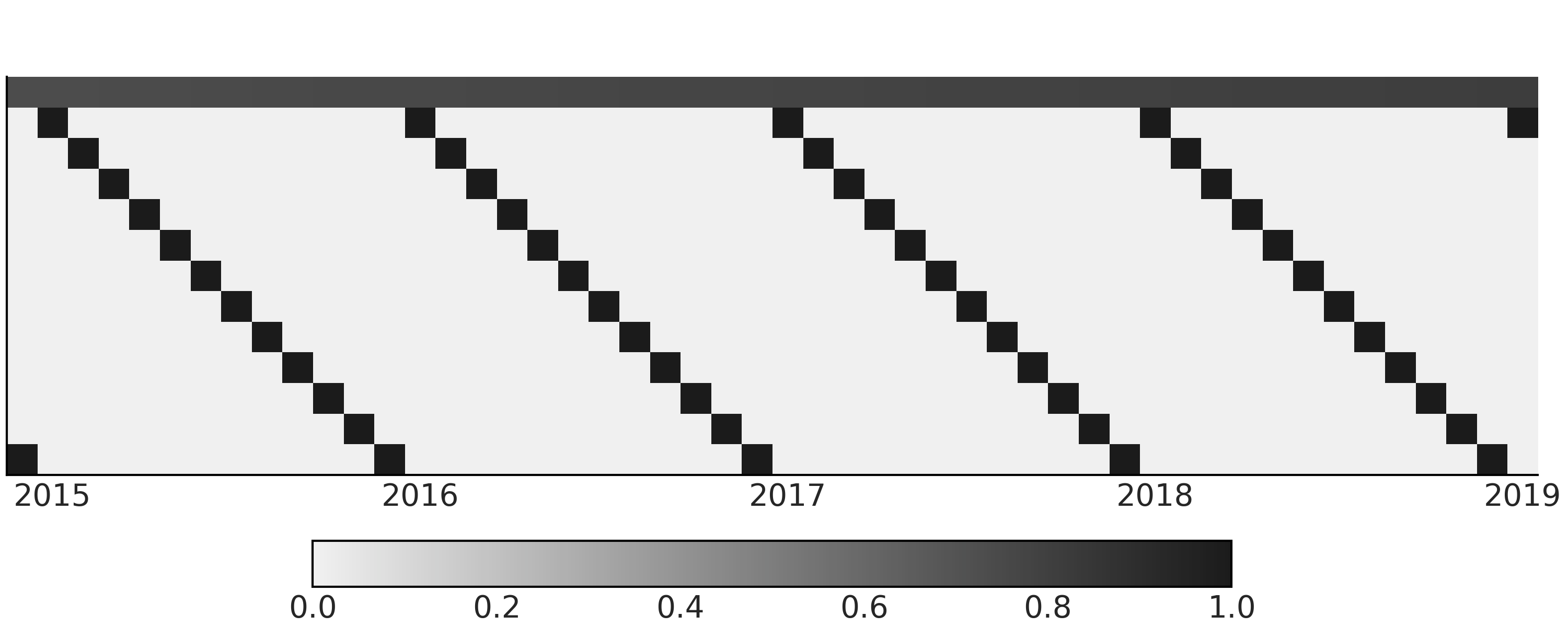
Fig. 6.2 Design matrix with a linear component and month of the year component for a simple regression model for time series. The design matrix is transposed into \(feature * timestamps\) so it is easier to visualize. In the figure, the first row (index 0) contains continuous values between 0 and 1 representing the time and the linear growth. The rest of the rows (index 1 - 12) are dummy coding of month information. The color coding goes from black for 1 to light gray for 0.#
trend_all = np.linspace(0., 1., len(co2_by_month))[..., None]
trend_all = trend_all.astype(np.float32)
trend = trend_all[:-num_forecast_steps, :]

seasonality_all = pd.get_dummies(
   co2_by_month.index.month).values.astype(np.float32)
seasonality = seasonality_all[:-num_forecast_steps, :]

_, ax = plt.subplots(figsize=(10, 4))
X_subset = np.concatenate([trend, seasonality], axis=-1)[-50:]
ax.imshow(X_subset.T)
We can now write down our first time series model as a regression
problem, using tfd.JointDistributionCoroutine, using the same
tfd.JointDistributionCoroutine API and TFP Bayesian modeling methods
we introduced in Chapter 3.
tfd = tfp.distributions
root = tfd.JointDistributionCoroutine.Root

@tfd.JointDistributionCoroutine
def ts_regression_model():
    intercept = yield root(tfd.Normal(0., 100., name="intercept"))
    trend_coeff = yield root(tfd.Normal(0., 10., name="trend_coeff"))
    seasonality_coeff = yield root(
        tfd.Sample(tfd.Normal(0., 1.),
                   sample_shape=seasonality.shape[-1],
                   name="seasonality_coeff"))
    noise = yield root(tfd.HalfCauchy(loc=0., scale=5., name="noise_sigma"))
    y_hat = (intercept[..., None] +
             tf.einsum("ij,...->...i", trend, trend_coeff) +
             tf.einsum("ij,...j->...i", seasonality, seasonality_coeff))
    observed = yield tfd.Independent(
        tfd.Normal(y_hat, noise[..., None]),
        reinterpreted_batch_ndims=1,
        name="observed")
As we mentioned in earlier chapters, TFP offers a lower level API
compared to PyMC3. While it is more flexible to interact with low level
modules and component (e.g., customized composable inference
approaches), we usually end up with a bit more boilerplate code, and
additional shape handling in the model using tfp compared to other
PPLs. For example, in Code Block
regression_model_for_timeseries
we use einsum instead of matmul with Python Ellipsis so it can
handle arbitrary batch shape (see Section Shape Handling in PPLs)
for more details).
Running the Code Block
regression_model_for_timeseries
gives us a regression model ts_regression_model. It has similar
functionality to tfd.Distribution which we can utilize in our Bayesian
workflow. To draw prior and prior predictive samples, we can call the
.sample(.) method (see Code Block
prior_predictive, with the result
shown in Fig. 6.3).
# Draw 100 prior and prior predictive samples
prior_samples = ts_regression_model.sample(100)
prior_predictive_timeseries = prior_samples.observed

fig, ax = plt.subplots(figsize=(10, 5))
ax.plot(co2_by_month.index[:-num_forecast_steps],
        tf.transpose(prior_predictive_timeseries), alpha=.5)
ax.set_xlabel("Year")
fig.autofmt_xdate()
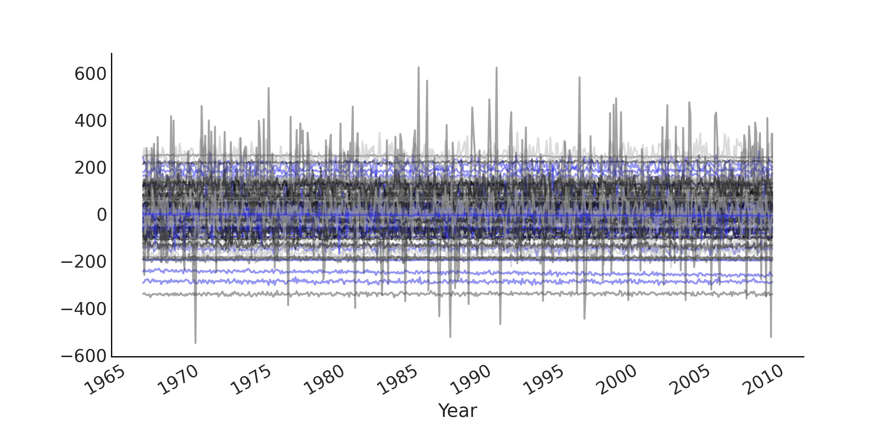
Fig. 6.3 Prior predictive samples from a simple regression model for modeling the Monthly CO₂ measurements in Mauna Loa time series. Each line plot is one simulated time series. Since we use an uninformative prior the prior prediction has a pretty wide range.#
We can now run inference of the regression model and format the result
into an az.InferenceData object in Code Block
inference_of_regression_model.
run_mcmc = tf.function(
    tfp.experimental.mcmc.windowed_adaptive_nuts,
    autograph=False, jit_compile=True)
mcmc_samples, sampler_stats = run_mcmc(
    1000, ts_regression_model, n_chains=4, num_adaptation_steps=1000,
    observed=co2_by_month_training_data["CO2"].values[None, ...])

regression_idata = az.from_dict(
    posterior={
        # TFP mcmc returns (num_samples, num_chains, ...), we swap
        # the first and second axis below for each RV so the shape
        # is what ArviZ expects.
        k:np.swapaxes(v.numpy(), 1, 0)
        for k, v in mcmc_samples._asdict().items()},
    sample_stats={
        k:np.swapaxes(sampler_stats[k], 1, 0)
        for k in ["target_log_prob", "diverging", "accept_ratio", "n_steps"]})
To draw posterior predictive samples conditioned on the inference
result, we can use the .sample_distributions method and condition on
the posterior samples. In this case, since we would like to also plot
the posterior predictive sample for the trend and seasonality components
in the time series, while conditioning on both the training and testing
data set. To visualize the forecasting ability of the model we construct
the posterior predictive distributions in Code Block
posterior_predictive_with_component,
with the result displayed in
Fig. 6.4 for the trend and
seasonality components and in Fig. 6.5
for the overall model fit and forecast.
# We can draw posterior predictive sample with jd.sample_distributions()
# But since we want to also plot the posterior predictive distribution for
# each components, conditioned on both training and testing data, we
# construct the posterior predictive distribution as below:
nchains = regression_idata.posterior.dims["chain"]

trend_posterior = mcmc_samples.intercept + \
    tf.einsum("ij,...->i...", trend_all, mcmc_samples.trend_coeff)
seasonality_posterior = tf.einsum(
    "ij,...j->i...", seasonality_all, mcmc_samples.seasonality_coeff)

y_hat = trend_posterior + seasonality_posterior
posterior_predictive_dist = tfd.Normal(y_hat, mcmc_samples.noise_sigma)
posterior_predictive_samples = posterior_predictive_dist.sample()
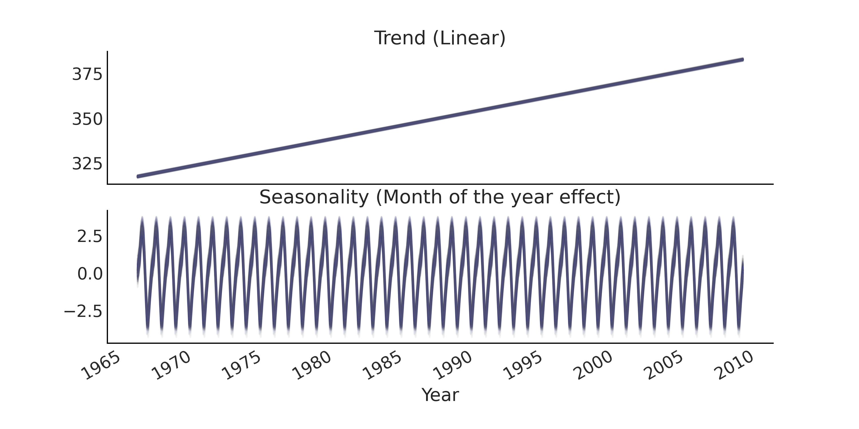
Fig. 6.4 Posterior predictive samples of the trend component and seasonality component of a regression model for time series.#
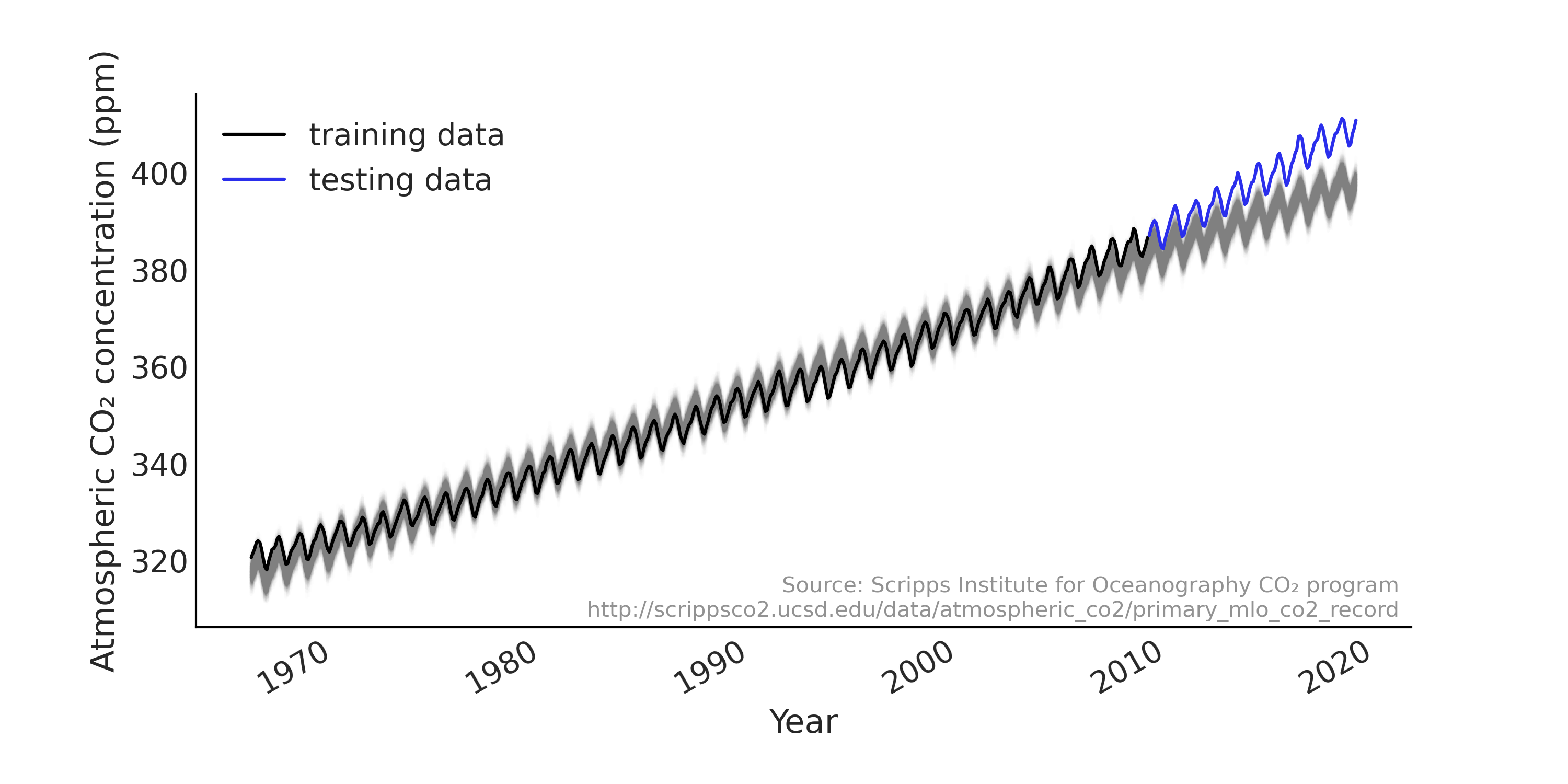
Fig. 6.5 Posterior predictive samples from a simple regression model for time series in gray, with the actual data plotted in black and blue. While the overall fit is reasonable for the training set (plotted in black), the forecast (out of sample prediction) is poor as the underlying trend is accelerating more than linearly.#
Looking at the out of sample prediction in Fig. 6.5, we notice that:
The linear trend does not perform well when we forecast further into the future and gives forecast consistently lower than the actual observed. Specifically the atmospheric CO₂ does not increase linearly with a constant slope over the years [4]
The range of uncertainty is almost constant (sometimes also referred to as the forecast cone), where intuitively we expect the uncertainty to increase when we forecast farther into the future.
6.2.1. Design Matrices for Time Series#
In the regression model above, a rather simplistic design matrix was used. We can get a better model to capture our knowledge of the observed time series by adding additional information to our design matrix.
Generally, a better trend component is the most important aspect for improving forecast performance: seasonality components are usually stationary [5] with easy to estimate parameters. Restated, there is a repeated pattern that forms a kind of a repeated measure. Thus most time series modeling involves designing a latent process that realistically captures the non-stationarity in the trend.
One approach that has been quite successful is using a local linear process for the trend component. Basically, it is a smooth trend that is linear within some range, with an intercept and coefficient that changes, or drifts, slowly over the observed time span. A prime example of such an application is Facebook Prophet [6], where a semi-smooth step linear function is used to model the trend [53]. By allowing the slope to change at some specific breakpoints, we can generate a trend line that could capture the long-term trend much better than a straight line. This is similar to the idea of indicator functions we discussed in Section Expanding the Feature Space. In a time series context we specify this idea mathematically in Equation (6.3)
where \(k\) is the (global) growth rate, \(\delta\) is a vector of rate
adjustments at each change point, \(m\) is the (global) intercept.
\(\mathbf{A}\) is a matrix with shape=(n_t, n_s) with \(n_s\) being the
number of change points. At time \(t\), \(\mathbf{A}\) accumulates the drift
effect \(\delta\) of the slope. \(\gamma\) is set to \(-s_j \times \delta_j\)
(where \(s_j\) is the time location of the \(n_s\) change points) to make
the trend line continuous. A regularized prior, like \(\text{Laplace}\),
is usually chosen for \(\delta\) to express that we don’t expect to see
sudden or large change in the slope. You can see in Code Block
step_linear_function_for_trend
for an example of a randomly generated step linear function and its
breakdown in Fig. 6.6.
n_changepoints = 8
n_tp = 500
t = np.linspace(0, 1, n_tp)
s = np.linspace(0, 1, n_changepoints + 2)[1:-1]
A = (t[:, None] > s)

k, m = 2.5, 40
delta = np.random.laplace(.1, size=n_changepoints)
growth = (k + A @ delta) * t
offset = m + A @ (-s * delta)
trend = growth + offset
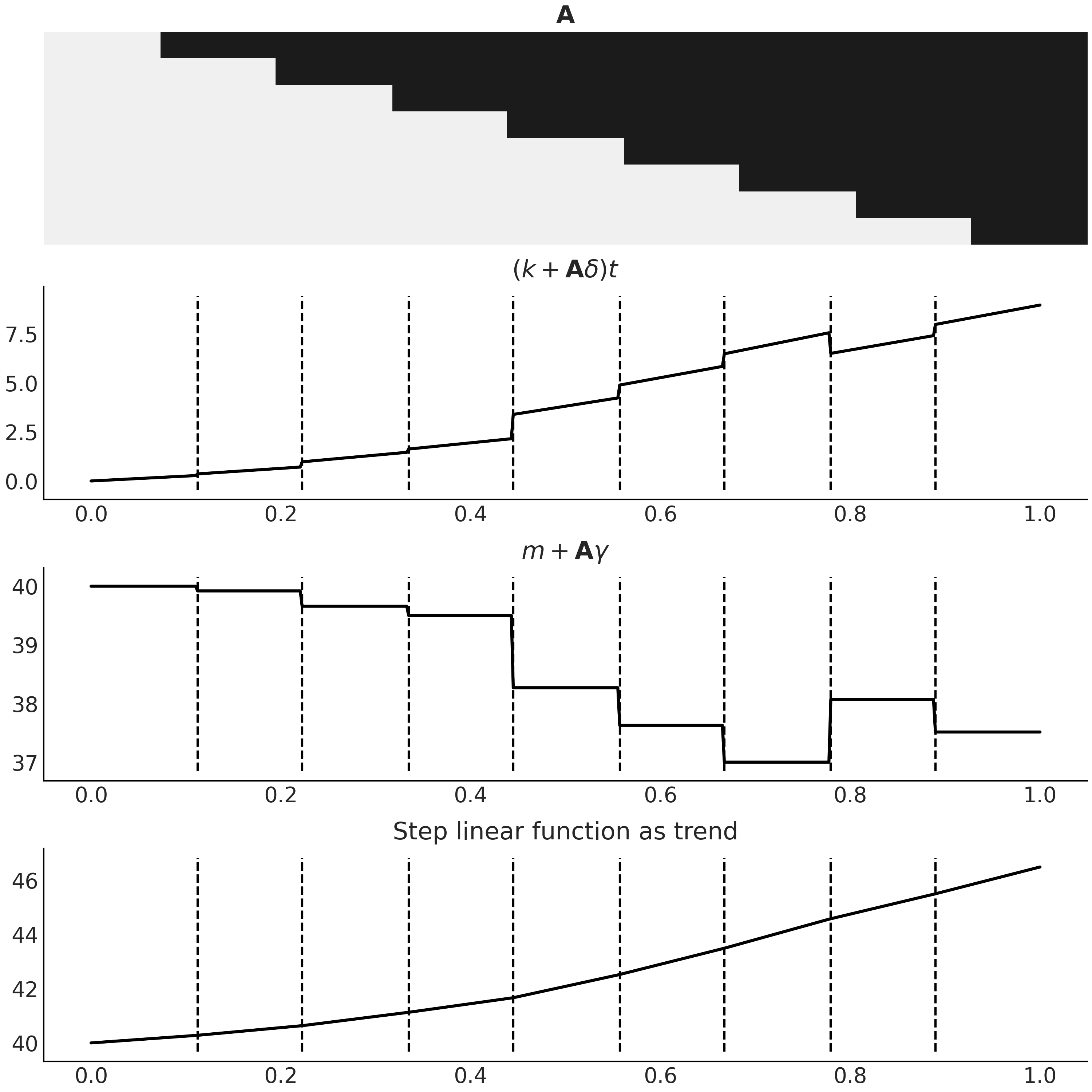
Fig. 6.6 A step linear function as trend component for a time series model, generated with Code Block step_linear_function_for_trend. The first panel is the design matrix \(\mathbf{A}\), with the same color coding that black for 1 and light gray for 0. The last panel is the resulting function \(g(t)\) in Equation (6.3) that we could use as trend in a time series model. The two middle panels are the breakdown of the two components in Equation (6.3). Note how combining the two makes the resulting trend continuous.#
In practice, we usually specify a priori how many change points there are so \(\mathbf{A}\) can be generated statically. One common approach is to specify more change points than you believe the time series actually displays, and place a more sparse prior on \(\delta\) to regulate the posterior towards 0. Automatic change point detection is also possible [54].
6.2.2. Basis Functions and Generalized Additive Model#
In our regression model defined in Code Block regression_model_for_timeseries, we model the seasonality component with a sparse, index, matrix. An alternative is to use basis functions like B-spline (see Chapter 5), or Fourier basis function as in the Facebook Prophet model. Basis function as a design matrix might provide some nice properties like orthogonality (see Box Mathematical properties of design matrix), which makes numerically solving the linear equation more stable [55].
Fourier basis functions are a collection of sine and cosine functions that can be used for approximating arbitrary smooth seasonal effects [56]:
where \(P\) is the regular period the time series has (e.g. \(P = 365.25\) for yearly data or \(P = 7\) for weekly data, when the time variable is scaled in days). We can generate them statically with formulation as shown in Code Block fourier_basis_as_seasonality, and visualize it in Fig. 6.7.
def gen_fourier_basis(t, p=365.25, n=3):
    x = 2 * np.pi * (np.arange(n) + 1) * t[:, None] / p
    return np.concatenate((np.cos(x), np.sin(x)), axis=1)

n_tp = 500
p = 12
t_monthly = np.asarray([i % p for i in range(n_tp)])
monthly_X = gen_fourier_basis(t_monthly, p=p, n=3)
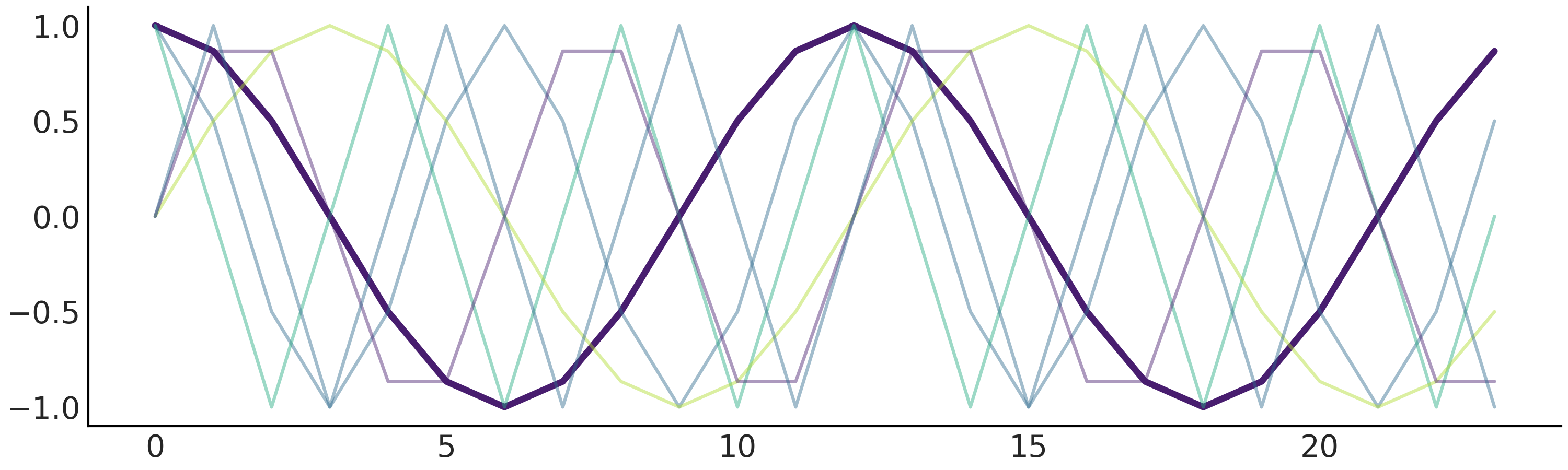
Fig. 6.7 Fourier basis function with n=3. There are in total 6 predictors, where we highlighted the first one by setting the rest semi-transparent.#
Fitting the seasonality using a design matrix generated from Fourier basis function as above requires estimating 2N parameters \(\beta = [a_1, b_1, \dots , a_N , b_N]\).
Regression models like Facebook Prophet are also referred to as a (GAM), as their response variable \(Y_t\) depends linearly on unknown smooth basis functions [7]. We also discussed other GAMs previously in Chapter 5.
Mathematical properties of design matrix
Mathematical properties of design matrices are studied quite extensively in the linear least squares problem setting, where we want to solve \(min \mid Y - \mathbf{X} \beta \mid ^{2}\) for \(\beta\). We can often get a sense how stable the solution of \(\beta\) will be, or even possible to get a solution at all, by inspecting the property of matrix \(\mathbf{X}^T \mathbf{X}\). One such property is the condition number, which is an indication of whether the solution of \(\beta\) may be prone to large numerical errors. For example, if the design matrix contains columns that are highly correlated (multicollinearity), the conditioned number will be large and the matrix \(\mathbf{X}^T \mathbf{X}\) is ill-conditioned. Similar principle also applies in Bayesian modeling. An in-depth exploratory data analysis in your analyses workflow is useful no matter what formal modeling approach you are taking. Basis functions as a design matrix usually are well-conditioned.
A Facebook Prophet-like GAM for the monthly CO₂ measurements is
expressed in Code Block gam. We assign weakly
informative prior to k and m to express our knowledge that monthly
measure is trending upward in general. This gives prior predictive
samples in a similar range of what is actually being observed (see
Fig. 6.8).
# Generate trend design matrix
n_changepoints = 12
n_tp = seasonality_all.shape[0]
t = np.linspace(0, 1, n_tp, dtype=np.float32)
s = np.linspace(0, max(t), n_changepoints + 2, dtype=np.float32)[1: -1]
A = (t[:, None] > s).astype(np.float32)
# Generate seasonality design matrix
# Set n=6 here so that there are 12 columns (same as `seasonality_all`)
X_pred = gen_fourier_basis(np.where(seasonality_all)[1],
                           p=seasonality_all.shape[-1],
                           n=6)
n_pred = X_pred.shape[-1]

@tfd.JointDistributionCoroutine
def gam():
    beta = yield root(tfd.Sample(
        tfd.Normal(0., 1.), sample_shape=n_pred, name="beta"))
    seasonality = tf.einsum("ij,...j->...i", X_pred, beta)

    k = yield root(tfd.HalfNormal(10., name="k"))
    m = yield root(tfd.Normal(
        co2_by_month_training_data["CO2"].mean(), scale=5., name="m"))
    tau = yield root(tfd.HalfNormal(10., name="tau"))
    delta = yield tfd.Sample(
        tfd.Laplace(0., tau), sample_shape=n_changepoints, name="delta")

    growth_rate = k[..., None] + tf.einsum("ij,...j->...i", A, delta)
    offset = m[..., None] + tf.einsum("ij,...j->...i", A, -s * delta)
    trend = growth_rate * t + offset

    y_hat = seasonality + trend
    y_hat = y_hat[..., :co2_by_month_training_data.shape[0]]

    noise_sigma = yield root(tfd.HalfNormal(scale=5., name="noise_sigma"))
    observed = yield tfd.Independent(
        tfd.Normal(y_hat, noise_sigma[..., None]),
        reinterpreted_batch_ndims=1,
        name="observed")
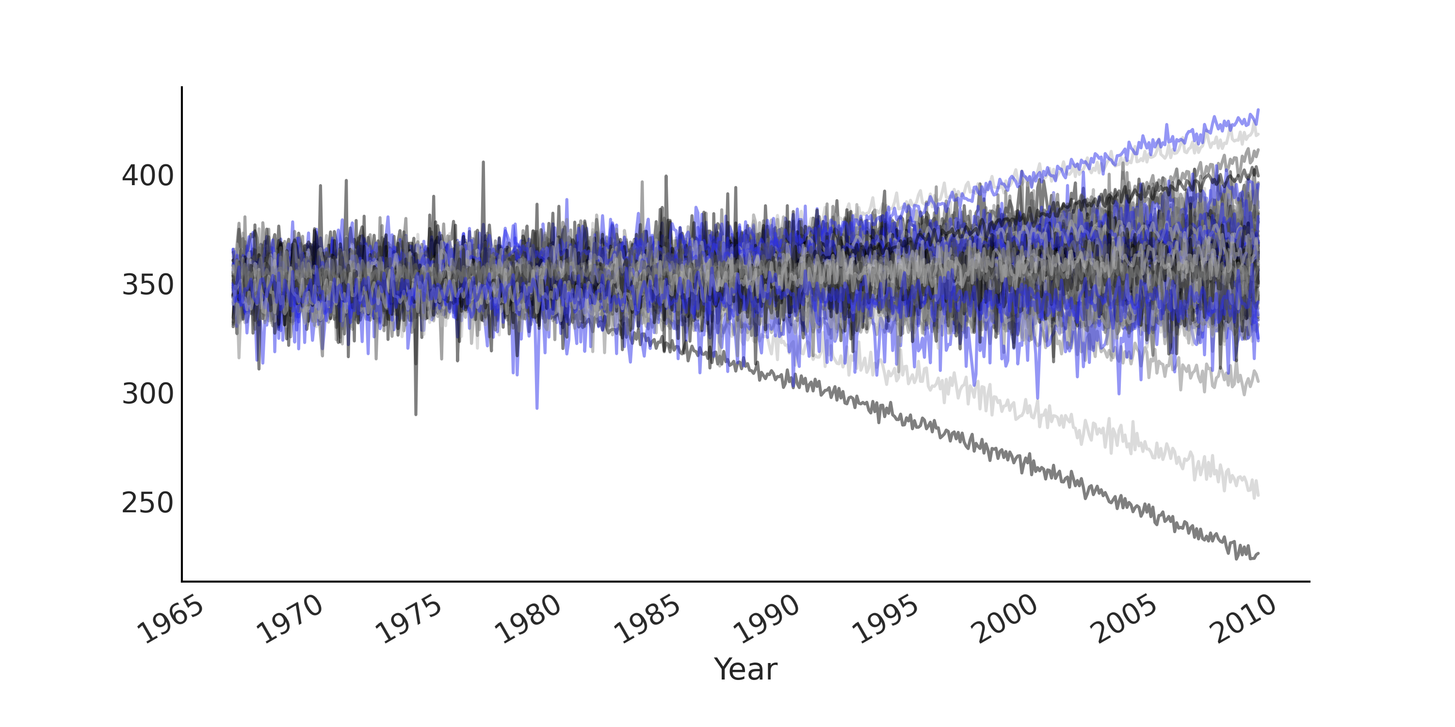
Fig. 6.8 Prior predictive samples from a Facebook Prophet-like GAM with a weakly informative prior on trend related parameters generated from Code Block gam. Each line plot is one simulated time series. The predictive samples are now in a similar range to what actually being observed, particularly when comparing this figure to Fig. 6.3.#
After inference, we can generate posterior predictive samples. As you can see in Fig. 6.9, the forecast performance is better than the simple regression model in Fig. 6.5. Note that in Taylor and Letham [53], the generative process for forecast is not identical to the generative model, as the step linear function is evenly spaced with the change point predetermined. It is recommended that for forecasting, at each time point we first determine whether that time point would be a change point, with a probability proportional to the number of predefined change points divided by the total number of observations, and then generate a new delta from the posterior distribution \(\delta_{new} \sim \text{Laplace}(0, \tau)\). Here however, to simplify the generative process we simply use the linear trend from the last period.
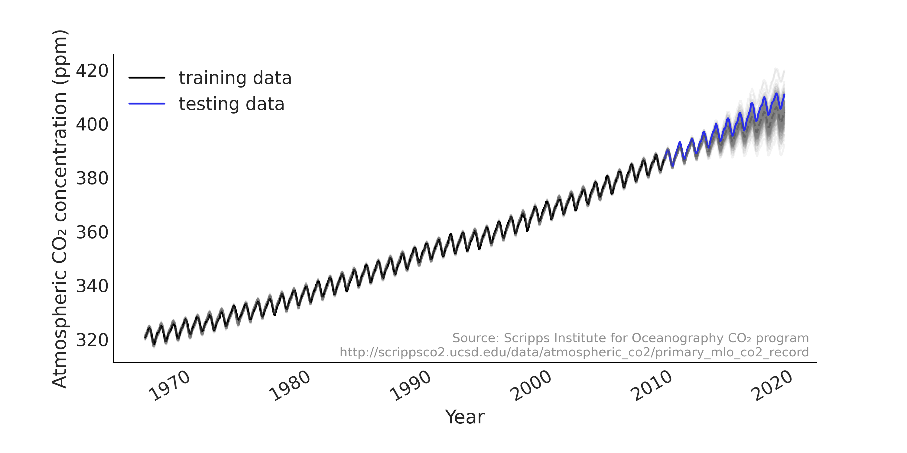
Fig. 6.9 Posterior predictive samples from a Facebook Prophet-like from Code Block gam in gray, with the actual data plotted in black and blue.#
6.3. Autoregressive Models#
One characteristic of time series is the sequential dependency of the observations. This usually introduces structured errors that are correlated temporally on previous observation(s) or error(s). A typical example is autoregressive-ness. In an autoregressive model, the distribution of output at time \(t\) is parameterized by a linear function of previous observations. Consider a first-order autoregressive model (usually we write that as AR(1) with a Gaussian likelihood:
The distribution of \(y_t\) follows a Normal distribution with the
location being a linear function of \(y_{t-1}\). In Python, we can write
down such a model with a for loop that explicitly builds out the
autoregressive process. For example, in Code Block
ar1_with_forloop we create an AR(1)
process using tfd.JointDistributionCoroutine with \(\alpha = 0\), and
draw random samples from it by conditioned on \(\sigma = 1\) and different
values of \(\rho\). The result is shown in
Fig. 6.10.
n_t = 200

@tfd.JointDistributionCoroutine
def ar1_with_forloop():
    sigma = yield root(tfd.HalfNormal(1.))
    rho = yield root(tfd.Uniform(-1., 1.))
    x0 = yield tfd.Normal(0., sigma)
    x = [x0]
    for i in range(1, n_t):
        x_i = yield tfd.Normal(x[i-1] * rho, sigma)
        x.append(x_i)

nplot = 4
fig, axes = plt.subplots(nplot, 1)
for ax, rho in zip(axes, np.linspace(-1.01, 1.01, nplot)):
    test_samples = ar1_with_forloop.sample(value=(1., rho))
    ar1_samples = tf.stack(test_samples[2:])
    ax.plot(ar1_samples, alpha=.5, label=r"$\rho$=%.2f" % rho)
    ax.legend(bbox_to_anchor=(1, 1), loc="upper left",
              borderaxespad=0., fontsize=10)
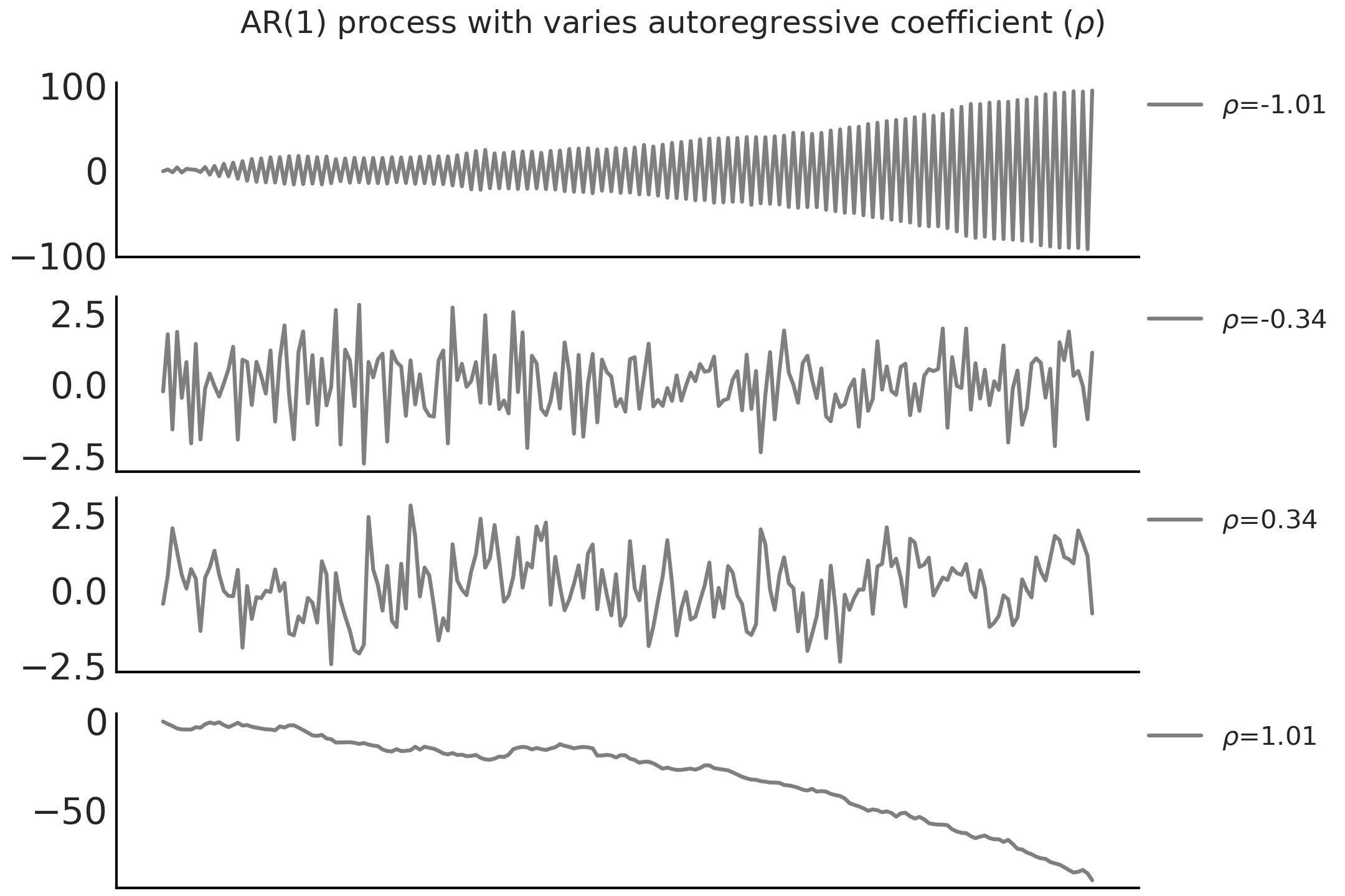
Fig. 6.10 Random sample of an AR(1) process with \(\sigma = 1\) and different \(\rho\). Note that the AR(1) process is not stationary when \(\mid \rho \mid > 1\).#
Using a for-loop to generate the time series random variable is pretty
straightforward, but now each time point is a random variable, which
makes working with it quite difficult (e.g., it does not scale well with
more time points). When possible, we prefer writing models that use
vectorized operations. The model above can be rewritten without using
for-loop by using the Autoregressive distribution tfd.Autoregressive
in TFP, which takes a distribution_fn that represents Equation
(6.5), a function that takes \(y_{t-1}\) as input and returns the
distribution of \(y_t\). However, the Autoregressive distribution in TFP
only retains the end state of the process, the distribution representing
the random variable \(y_t\) after the initial value \(y_0\) iterates for \(t\)
steps. To get all the time steps of a AR process, we need to express
Equation (6.5) a bit differently using a backshift operator, also
called (Lag operator) \(\mathbf{B}\) that shifts the time series
\(\mathbf{B} y_t = y_{t-1}\) for all \(t > 0\). Re-expressing Equation
(6.5) with a backshift operator \(\mathbf{B}\) we have
\(Y \sim \mathcal{N}(\rho \mathbf{B} Y, \sigma)\). Conceptually, you can
think of it as evaluating a vectorized likelihood
Normal(ρ * y[:-1], σ).log_prob(y[1:]). In Code Block
ar1_without_forloop we construct
the same generative AR(1) model for n_t steps with the
tfd.Autoregressive API. Note that we did not construct the backshift
operator \(\mathbf{B}\) explicitly by just generating the outcome
\(y_{t-1}\) directly shown in Code Block
ar1_without_forloop, where a Python
function ar1_fun applies the backshift operation and generates the
distribution for the next step.
@tfd.JointDistributionCoroutine
def ar1_without_forloop():
    sigma = yield root(tfd.HalfNormal(1.))
    rho = yield root(tfd.Uniform(-1., 1.))

    def ar1_fun(x):
        # We apply the backshift operation here
        x_tm1 = tf.concat([tf.zeros_like(x[..., :1]), x[..., :-1]], axis=-1)
        loc = x_tm1 * rho[..., None]
        return tfd.Independent(tfd.Normal(loc=loc, scale=sigma[..., None]),
                               reinterpreted_batch_ndims=1)

    dist = yield tfd.Autoregressive(
        distribution_fn=ar1_fun,
        sample0=tf.zeros([n_t], dtype=rho.dtype),
        num_steps=n_t)
We are now ready to extend the Facebook Prophet -like GAM above with AR(1) process as likelihood. But before we do that let us rewrite the GAM in Code Block gam slightly differently into Code Block gam_alternative.
def gam_trend_seasonality():
    beta = yield root(tfd.Sample(
        tfd.Normal(0., 1.), sample_shape=n_pred, name="beta"))
    seasonality = tf.einsum("ij,...j->...i", X_pred, beta)

    k = yield root(tfd.HalfNormal(10., name="k"))
    m = yield root(tfd.Normal(
        co2_by_month_training_data["CO2"].mean(), scale=5., name="m"))
    tau = yield root(tfd.HalfNormal(10., name="tau"))
    delta = yield tfd.Sample(
        tfd.Laplace(0., tau), sample_shape=n_changepoints, name="delta")

    growth_rate = k[..., None] + tf.einsum("ij,...j->...i", A, delta)
    offset = m[..., None] + tf.einsum("ij,...j->...i", A, -s * delta)
    trend = growth_rate * t + offset
    noise_sigma = yield root(tfd.HalfNormal(scale=5., name="noise_sigma"))
    return seasonality, trend, noise_sigma

def generate_gam(training=True):

    @tfd.JointDistributionCoroutine
    def gam():
        seasonality, trend, noise_sigma = yield from gam_trend_seasonality()
        y_hat = seasonality + trend
        if training:
            y_hat = y_hat[..., :co2_by_month_training_data.shape[0]]

        # likelihood
        observed = yield tfd.Independent(
            tfd.Normal(y_hat, noise_sigma[..., None]),
            reinterpreted_batch_ndims=1,
            name="observed"
        )

    return gam

gam = generate_gam()
Comparing Code Block gam_alternative with Code Block gam, we see two major differences:
We split out the construction of the trend and seasonality components (with their priors) into a separate function, and in the
tfd.JointDistributionCoroutinemodel block we use ayield fromstatement so we get the identicaltfd.JointDistributionCoroutinemodel in both Code Blocks;We wrap the
tfd.JointDistributionCoroutinein another Python function so it is easier to condition on both the training and testing set.
Code Block gam_alternative is a much more modular approach. We can write down a GAM with an AR(1) likelihood by just changing the likelihood part. This is what we do in Code Block gam_with_ar_likelihood.
def generate_gam_ar_likelihood(training=True):

    @tfd.JointDistributionCoroutine
    def gam_with_ar_likelihood():
        seasonality, trend, noise_sigma = yield from gam_trend_seasonality()
        y_hat = seasonality + trend
        if training:
            y_hat = y_hat[..., :co2_by_month_training_data.shape[0]]

        # Likelihood
        rho = yield root(tfd.Uniform(-1., 1., name="rho"))
        def ar_fun(y):
            loc = tf.concat([tf.zeros_like(y[..., :1]), y[..., :-1]],
                            axis=-1) * rho[..., None] + y_hat
            return tfd.Independent(
                tfd.Normal(loc=loc, scale=noise_sigma[..., None]),
                reinterpreted_batch_ndims=1)
        observed = yield tfd.Autoregressive(
            distribution_fn=ar_fun,
            sample0=tf.zeros_like(y_hat),
            num_steps=1,
            name="observed")

    return gam_with_ar_likelihood

gam_with_ar_likelihood = generate_gam_ar_likelihood()
Another way to think about AR(1) model here is as extending our linear regression notion to include an observation dependent column in the design matrix, and setting the element of this column \(x_i\) being \(y_{i-1}\). The autoregressive coefficient \(\rho\) is then no different to any other regression coefficient, which is just telling us what is the linear contribution of the previous observation to the expectation of the current observation [8]. In this model, we found that the effect is almost negligible by inspecting the posterior distribution of \(\rho\) (see Fig. 6.11):
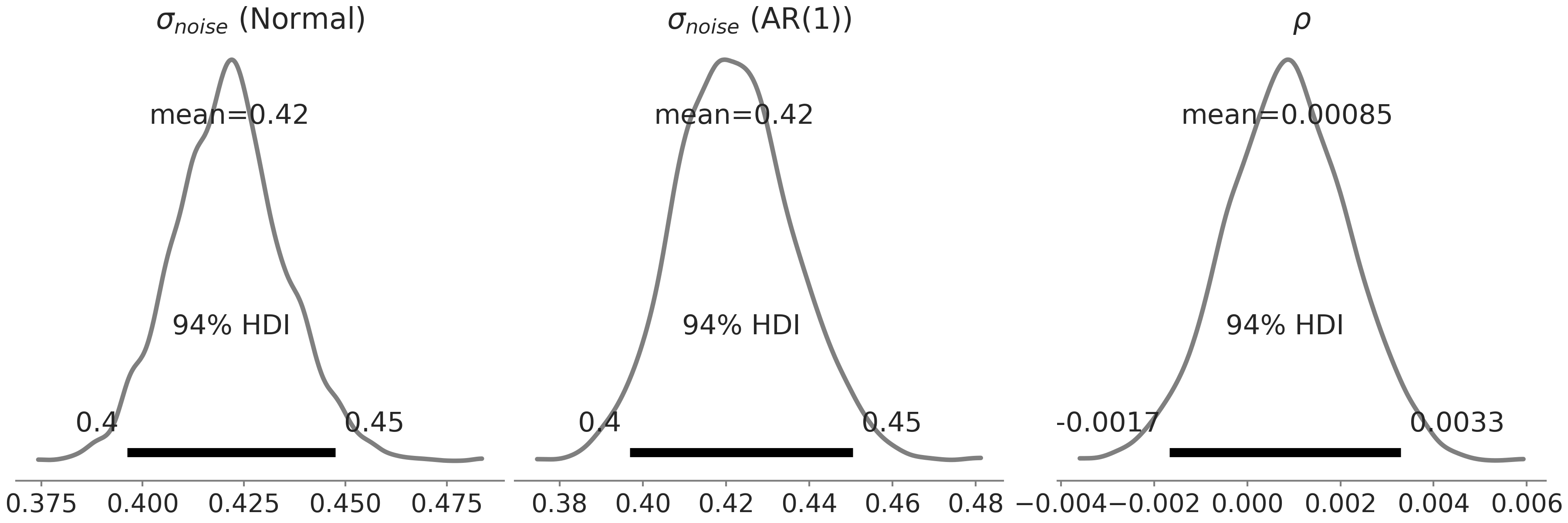
Fig. 6.11 Posterior distribution of the parameters in the likelihood for the Facebook Prophet -like GAM defined in Code Block gam_with_ar_likelihood. Leftmost panel is the \(\sigma\) in the model with a Normal likelihood, middle and rightmost panels are \(\sigma\) and \(\rho\) in the model with an AR(1) likelihood. Both models return a similar estimation of \(\sigma\), with the \(\rho\) estimated centered around 0.#
Instead of using an AR(k) likelihood, we can also include AR in a time
series model by adding a latent AR component to the linear prediction.
This is the gam_with_latent_ar model in Code Block
gam_with_latent_ar.
def generate_gam_ar_latent(training=True):

    @tfd.JointDistributionCoroutine
    def gam_with_latent_ar():
        seasonality, trend, noise_sigma = yield from gam_trend_seasonality()

        # Latent AR(1)
        ar_sigma = yield root(tfd.HalfNormal(.1, name="ar_sigma"))
        rho = yield root(tfd.Uniform(-1., 1., name="rho"))
        def ar_fun(y):
            loc = tf.concat([tf.zeros_like(y[..., :1]), y[..., :-1]],
                            axis=-1) * rho[..., None]
            return tfd.Independent(
                tfd.Normal(loc=loc, scale=ar_sigma[..., None]),
                reinterpreted_batch_ndims=1)
        temporal_error = yield tfd.Autoregressive(
            distribution_fn=ar_fun,
            sample0=tf.zeros_like(trend),
            num_steps=trend.shape[-1],
            name="temporal_error")

        # Linear prediction
        y_hat = seasonality + trend + temporal_error
        if training:
            y_hat = y_hat[..., :co2_by_month_training_data.shape[0]]

        # Likelihood
        observed = yield tfd.Independent(
            tfd.Normal(y_hat, noise_sigma[..., None]),
            reinterpreted_batch_ndims=1,
            name="observed"
        )

    return gam_with_latent_ar

gam_with_latent_ar = generate_gam_ar_latent()
With the explicit latent AR process, we are adding a random variable with the same size as the observed data to the model. Since it is now an explicit component added to the linear prediction \(\hat{Y}\), we can interpret the AR process to be complementary to, or even part of, the trend component. We can visualize the latent AR component after inference similar to the trend and seasonality components of a time series model (see Fig. 6.12).
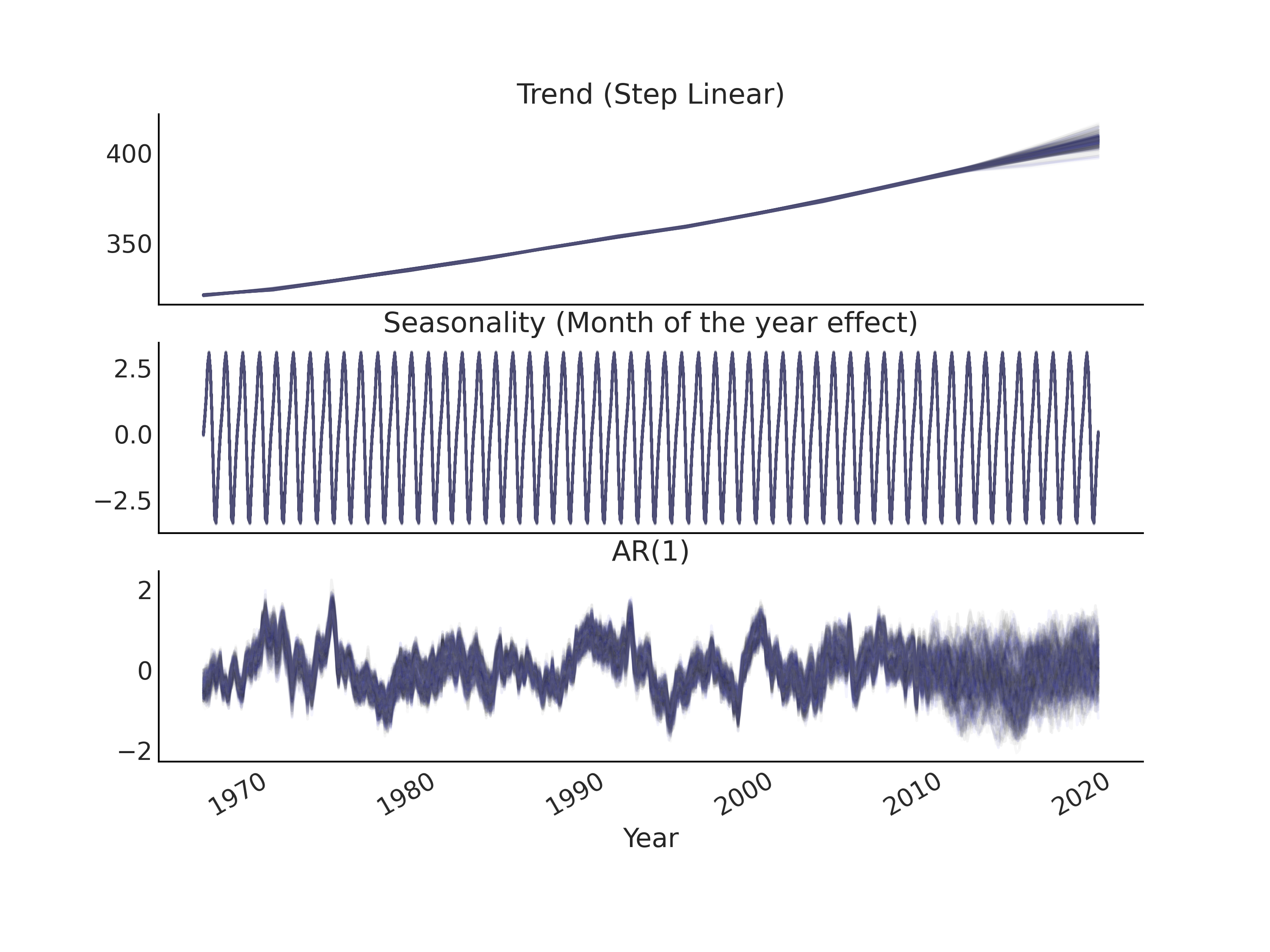
Fig. 6.12 Posterior predictive samples of the trend, seasonality, and AR(1)
components of the GAM based time series model gam_with_latent_ar
specified in Code Block
gam_with_latent_ar.#
Another way to interpret the explicit latent AR process is that it
captures the temporally correlated residuals, so we expect the
posterior estimation of the \(\sigma_{noise}\) will be smaller compared to
the model without this component. In
Fig. 6.13 we display the posterior
distribution of \(\sigma_{noise}\), \(\sigma_{AR}\), and \(\rho\) for model
gam_with_latent_ar. In comparison to model gam_with_ar_likelihood,
we indeed get a lower estimation of \(\sigma_{noise}\), with a much higher
estimation of \(\rho\).
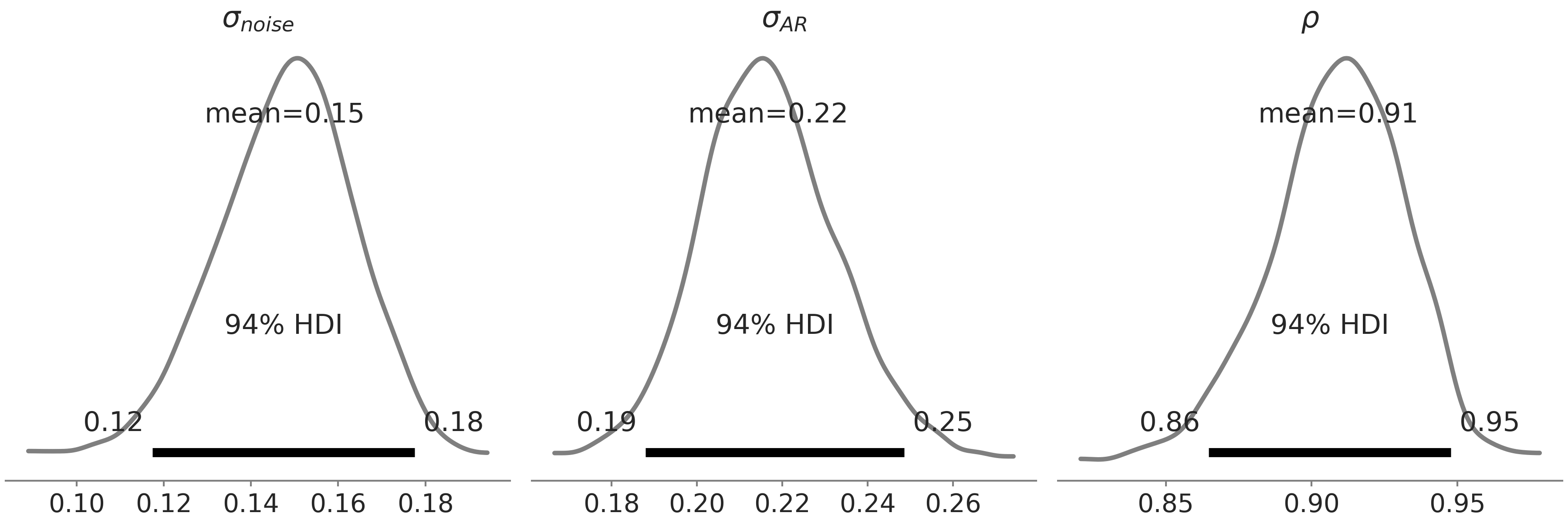
Fig. 6.13 Posterior distribution of \(\sigma_{noise}\), \(\sigma_{AR}\), and \(\rho\) of
the AR(1) latent component for gam_with_latent_ar specified in Code
Block gam_with_latent_ar. Note not
to be confused with Fig. 6.11 where we
displays posterior distribution of parameters from 2 different GAMs.#
6.3.1. Latent AR Process and Smoothing#
A latent process is quite powerful at capturing the subtle trends in the observed time series. It can even approximate some arbitrary functions. To see that let us consider modeling a toy problem with a time series model that contains a latent (GRW) component, as formulated in Equation (6.6).
The GRW here is the same as an AR(1) process with \(\rho = 1\). By placing different prior on \(\sigma_{z}\) and \(\sigma_{y}\) in Equation (6.6), we can emphasize how much of the variance in the observed data should be accounted for in the GRW, and how much is iid noise. We can also compute the ratio \(\alpha = \frac{\sigma_{y}^2}{\sigma_{z}^2 + \sigma_{y}^2}\), where \(\alpha\) is in the range \([0, 1]\) that can be interpret as the degree of smoothing. Thus we can express the model in Equation (6.6) equivalently as Equation (6.7).
Our latent GRW model in Equation (6.7) could be
written in TFP in Code Block gw_tfp. By placing
informative prior on \(\alpha\) we can control how much “smoothing” we
would like to see in the latent GRW (larger \(\alpha\) gives smoother
approximation). Let us fit the model smoothing_grw with some noisy
observations simulated from an arbitrary function. The data is shown as
black solid dots in Fig. 6.14, with the
fitted latent Random Walk displayed in the same Figure. As you can see
we can approximate the underlying function pretty well.
@tfd.JointDistributionCoroutine
def smoothing_grw():
    alpha = yield root(tfd.Beta(5, 1.))
    variance = yield root(tfd.HalfNormal(10.))
    sigma0 = tf.sqrt(variance * alpha)
    sigma1 = tf.sqrt(variance * (1. - alpha))
    z = yield tfd.Sample(tfd.Normal(0., sigma0), num_steps)
    observed = yield tfd.Independent(
        tfd.Normal(tf.math.cumsum(z, axis=-1), sigma1[..., None]))
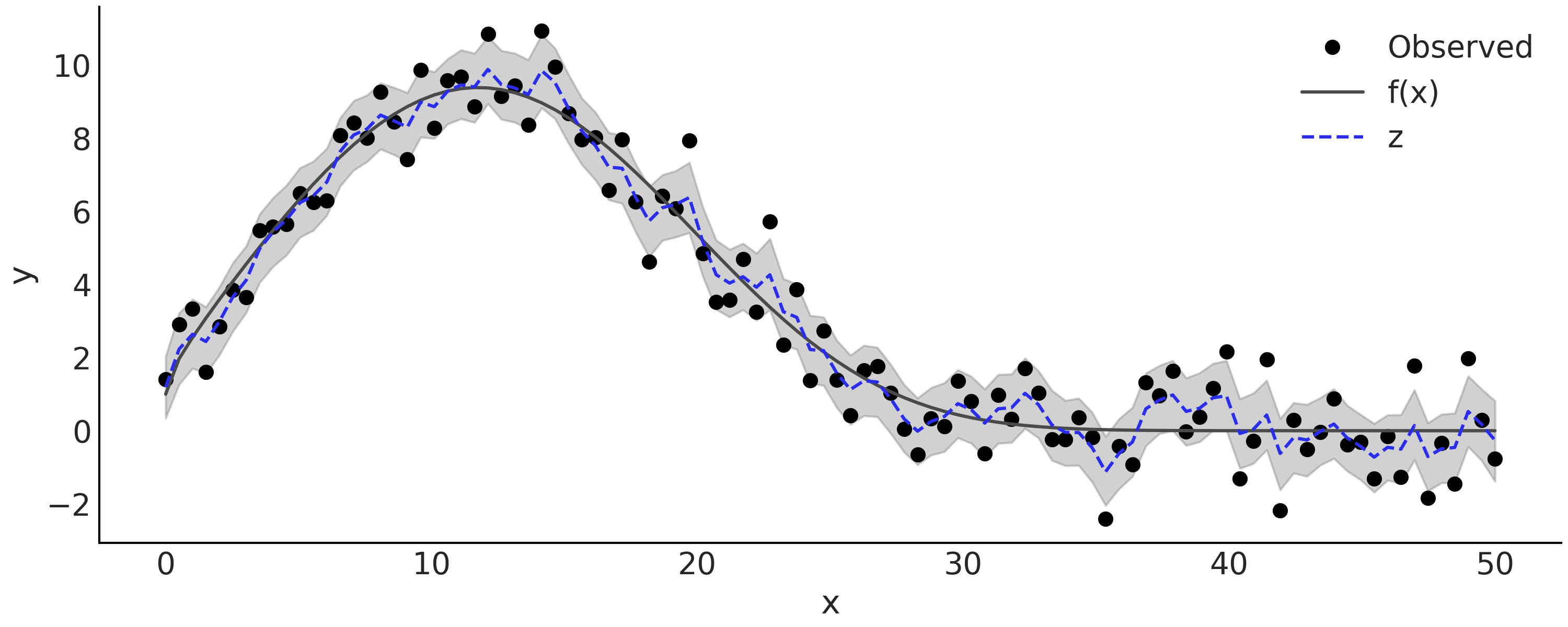
Fig. 6.14 Simulated observations from \(y \sim \text{Normal}(f(x), 1)\) with \(f(x) = e^{1 + x^{0.5} - e^{\frac{x}{15}}}\), and the inferred latent Gaussian Random Walk. The gray semi-transparent region is the posterior 94% HDI interval of the latent Gaussian Random Walk \(z\), with the posterior mean plot in dash blue line.#
There are a few other interesting properties of the AR process, with connection to the Gaussian Process [52]. For example, you might find that the Autoregressive model alone is useless to capture the long-term trend. Even though the model seems to fit well the observation, during forecast you will observe the forecast value regress to the mean of the last few time steps very quickly. Same as what you will observe using the Gaussian Process with a constant mean function [9].
An autoregressive component as an additional trend component could place some challenges to model inference. For example, scaling could be an issue as we are adding a random variable with the same shape as the observed time series. We might have an unidentifiable model when both the trend component and the AR process are flexible, as the AR process alone already has the ability to approximate the underlying trend, a smoothed function, of the observed data as we have seen here.
6.3.2. (S)AR(I)MA(X)#
Many classical time series models share a similar autoregressive like pattern, where you have some latent parameter at time \(t\) that is dependent on the value of itself or another parameter at \(t-k\). Two examples of these models are
Autoregressive conditional heteroscedasticity (ARCH) model, where the scale of the residuals vary over time;
Moving average (MA) model, which is a linear combination of previous residuals are added to the mean of the series.
Some of these classical time series models could be combined into more complex models, one of such extensions is the Seasonal AutoRegressive Integrated Moving Average with eXogenous regressors model (SARIMAX). While the naming might look intimidating, the basic concept is largely a straightforward combination of the AR and MA model. Extending the AR model with MA we get:
where \(p\) is the order of the autoregressive model and \(q\) is the order of the moving average model. Conventionally, we write models as such being ARMA(p, q). Similarly, for seasonal ARMA we have:
The integrated part of an ARIMA model refers to the summary statistics
of a time series: order of integration. Denoted as \(I(d)\), a time series
is integrated to order \(d\) if taking repeated differences \(d\) times
yields a stationary series. Following Box et al. [57],
we repeatedly take difference of the observed time series as a
preprocessing step to account for the \(I(d)\) part of an ARIMA(p,d,q)
model, and model the resulting differenced series as a stationary
process with ARMA(p,q). The operation itself is also quite standard in
Python. We can use numpy.diff where the first difference computed is
delta_y[i] = y[i] - y[i-1] along a given axis, and higher differences
are calculated by repeating the same operation recursively on the
resulting array.
If we have an additional regressor \(\mathbf{X}\), in the model above \(\alpha\) is replaced with the linear prediction \(\mathbf{X} \beta\). We will apply the same differencing operation on \(\mathbf{X}\) if \(d > 0\). Note that we can have either seasonal (SARIMA) or exogenous regressors (ARIMAX) but not both.
Notation for (S)AR(I)MA(X)
Typically, ARIMA models are denoted as ARIMA(p,d,q), which is to say we have a model containing order \(p\) of AR, \(d\) degree of I, and order \(q\) of MA. For example, ARIMA(1,0,0) is just a AR(1). We denote seasonal ARIMA models as \(\text{SARIMA}(p,d,q)(P,D,Q)_{s}\), where \(s\) refers to the number of periods in each season, and the uppercase \(P\), \(D\), \(Q\) are the seasonal counter part of the ARIMA model \(p\), \(d\), \(q\). Sometimes seasonal ARIMA are denoted also as \(\text{SARIMA}(p,d,q)(P,D,Q,s)\). If there are exogenous regressors, we write \(\text{ARIMAX}(p,d,q)\mathbf{X}[k]\) with \(\mathbf{X}[k]\) indicating we have a \(k\) columns design matrix \(\mathbf{X}\).
As the second example in this chapter, we will use different ARIMA to model the time series of the monthly live births in the United States from 1948 to 1979 [58]. The data is shown in Fig. 6.15.
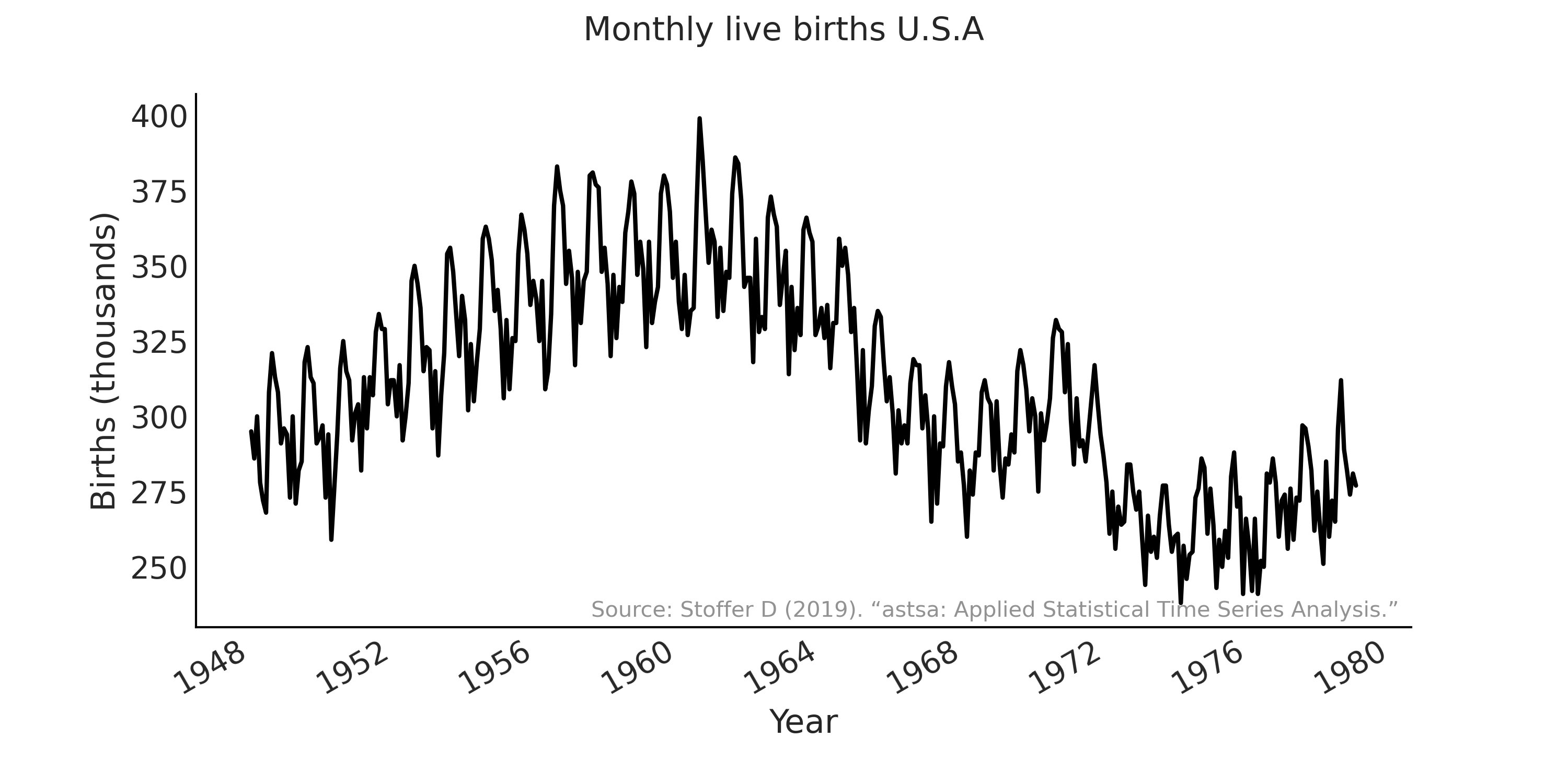
Fig. 6.15 Monthly live births in the United States (1948-1979). Y-axis shows the number of births in thousands.#
We will start with a \(\text{SARIMA}(1, 1, 1)(1, 1, 1)_{12}\) model. First we load and pre-process the observed time series in Code Block sarima_preprocess.
us_monthly_birth = pd.read_csv("../data/monthly_birth_usa.csv")
us_monthly_birth["date_month"] = pd.to_datetime(us_monthly_birth["date_month"])
us_monthly_birth.set_index("date_month", drop=True, inplace=True)

# y ~ Sarima(1,1,1)(1,1,1)[12]
p, d, q = (1, 1, 1)
P, D, Q, period = (1, 1, 1, 12)
# Time series data: us_monthly_birth.shape = (372,)
observed = us_monthly_birth["birth_in_thousands"].values
# Integrated to seasonal order $D$
for _ in range(D):
    observed = observed[period:] - observed[:-period]
# Integrated to order $d$
observed = tf.constant(np.diff(observed, n=d), tf.float32)
At time of writing TFP does not have a dedicated implementation of an
ARMA distribution. To run inference of our SARIMA model, TFP requires a
Python callable representing the log posterior density function (up to
some constant [30]. In this case, we can archive that by
implementing the likelihood function of \(\text{SARMA}(1, 1)(1, 1)_{12}\)
(since the \(\text{I}\) part is already dealt with via differencing). We
do that in Code Block
sarima_likelihood using a
tf.while_loop to construct the residual time series \(\epsilon_t\) and
evaluated on a \(\text{Normal}\) distribution [10]. From the programming
point of view, the biggest challenge here is to make sure the shape is
correct when we index to the time series. To avoid additional control
flow to check whether some of the indexes are valid (e.g, we cannot
index to \(t-1\) and \(t-period-1\) when \(t=0\)), we pad the time series with
zeros.
def likelihood(mu0, sigma, phi, theta, sphi, stheta):
    batch_shape = tf.shape(mu0)
    y_extended = tf.concat(
        [tf.zeros(tf.concat([[r], batch_shape], axis=0), dtype=mu0.dtype),
        tf.einsum("...,j->j...",
                  tf.ones_like(mu0, dtype=observed.dtype),
                  observed)],
        axis=0)
    eps_t = tf.zeros_like(y_extended, dtype=observed.dtype)

    def arma_onestep(t, eps_t):
        t_shift = t + r
        # AR
        y_past = tf.gather(y_extended, t_shift - (np.arange(p) + 1))
        ar = tf.einsum("...p,p...->...", phi, y_past)
        # MA
        eps_past = tf.gather(eps_t, t_shift - (np.arange(q) + 1))
        ma = tf.einsum("...q,q...->...", theta, eps_past)
        # Seasonal AR
        sy_past = tf.gather(y_extended, t_shift - (np.arange(P) + 1) * period)
        sar = tf.einsum("...p,p...->...", sphi, sy_past)
        # Seasonal MA
        seps_past = tf.gather(eps_t, t_shift - (np.arange(Q) + 1) * period)
        sma = tf.einsum("...q,q...->...", stheta, seps_past)

        mu_at_t = ar + ma + sar + sma + mu0
        eps_update = tf.gather(y_extended, t_shift) - mu_at_t
        epsilon_t_next = tf.tensor_scatter_nd_update(
            eps_t, [[t_shift]], eps_update[None, ...])
        return t+1, epsilon_t_next

    t, eps_output_ = tf.while_loop(
        lambda t, *_: t < observed.shape[-1],
        arma_onestep,
        loop_vars=(0, eps_t),
        maximum_iterations=observed.shape[-1])
    eps_output = eps_output_[r:]
    return tf.reduce_sum(
        tfd.Normal(0, sigma[None, ...]).log_prob(eps_output), axis=0)
Adding the prior to the unknown parameters (in this case, mu0,
sigma, phi, theta, sphi, and stheta), we can generate the
posterior density function for inference. This is shown in Code Block
sarima_posterior, with a resulting
target_log_prob_fn that we sample from in Code Block
sarima_posterior [11].
@tfd.JointDistributionCoroutine
def sarima_priors():
    mu0 = yield root(tfd.StudentT(df=6, loc=0, scale=2.5, name='mu0'))
    sigma = yield root(tfd.HalfStudentT(df=7, loc=0, scale=1., name='sigma'))

    phi = yield root(tfd.Sample(tfd.Normal(0, 0.5), p, name='phi'))
    theta = yield root(tfd.Sample(tfd.Normal(0, 0.5), q, name='theta'))
    sphi = yield root(tfd.Sample(tfd.Normal(0, 0.5), P, name='sphi'))
    stheta = yield root(tfd.Sample(tfd.Normal(0, 0.5), Q, name='stheta'))

target_log_prob_fn = lambda *x: sarima_priors.log_prob(*x) + likelihood(*x)
The preprocessing of the time series to account for the integrated
part in Code Block sarima_preprocess
and the likelihood implementation in Code Block
sarima_likelihood could be refactored
into a helper Python Class that flexibility generate different SARIMA
likelihood. For example, Table 6.1 shows the model
comparison between the \(\text{SARIMA}(1,1,1)(1,1,1)_{12}\) model from
Code Block sarima_posterior and a
similar \(\text{SARIMA}(0,1,2)(1,1,1)_{12}\) model.
rank |
loo |
p_loo |
d_loo |
weight |
se |
dse |
|
\(\text{SARIMA}(0,1,2)(1,1,1)_{12}\) |
0 |
-1235.60 |
7.51 |
0.00 |
0.5 |
15.41 |
0.00 |
\(\text{SARIMA}(1,1,1)(1,1,1)_{12}\) |
1 |
-1235.97 |
8.30 |
0.37 |
0.5 |
15.47 |
6.29 |
6.4. State Space Models#
In the implementation of the ARMA log-likelihood function above (Code Block sarima_likelihood), we iterate through time steps to condition on the observations and construct some latent variables for that time slice. Indeed, unless the models are of a very specific and simple variety (e.g. the Markov dependencies between each two consecutive time steps make it possible to reduce the generative process into vectorized operations), this recursive pattern is a very natural way to express time series models. A powerful, general formulation of this pattern is the State Space model, a discrete-time process where we assume at each time step some latent states \(X_t\) evolves from previous step \(X_{t-1}\) (a Markov Sequence), and we observed \(Y_t\) that is some projection from the latent states \(X_t\) to the observable space [12]:
where \(p(X_0)\) is the prior distribution of the latent states at time step 0, \(p^{\theta}(X_{t+1} \mid X_t)\) is the transition probability distribution parameterized by a vector of parameter \(\theta\) that describes the system dynamics, and \(p^{\psi}(Y_t \mid X_t)\) being the observation distribution parameterized by \(\psi\) that describes the measurement at time \(t\) conditioned on the latent states.
Implementation of state space model for efficient computation
There is a harmony between mathematical formulation and computation implementation
of a State Space model with API like tf.while_loop or tf.scan.
Unlike using a Python for loop or while loop, they require compiling
the loop body into a function that takes the same structure of tensors
as input and outputs. This functional style of implementation is useful
to make explicit how the latent states are being transitioned at each
time step and how the measurement, from latent state to observed, should
be outputted. It is worth noting that implementation of state space
model and its associated inference algorithm like Kalman filter also
involved design decisions about where to place some of the initial
computation. In the formulation above, we place a prior on the initial
latent condition, and the first observation is a measure of the initial
state directly. However, it is equally valid to make a transition on the
latent state at step 0, then make the first observation with
modification to the prior distribution the two approaches are
equivalent.
There is however a subtle trickiness in dealing with shape when
implementing filters for time series problems. The main challenge is
where to place the time dimension. An obvious choice is to place it at
axis 0, as it becomes nature to do time_series[t] with t being some
time index. Moreover, loop construction using tf.scan or theano.scan
to loop over a time series automatically places the time dimension on
axis 0. However, it conflicts with the batch dimensions, which are
usually the leading axis. For example, if we want to vectorize over N
batch of k dimension time series, each with T total time stamps, the
array will have a shape of [N, T, ...] but the output of tf.scan
will have a shape of [T, N, ...]. Currently, it seems unavoidable that
modelers need to perform some transpose on a scan output so that it
matches the semantic of the batch and time dimension as the input.
Once we have the state space representation of a time series problem, we are in a sequential analysis framework that typically includes tasks like filtering and smoothing:
Filtering: computing the marginal distribution of the latent state \(X_k\), conditioned on observations up to that time step \(k\): \(p(X_k \mid y_{0:k}), k = 0,...,T\); \(\circ\) Prediction: a forecast distribution of the latent state, extending the filtering distribution into the future for \(n\) steps: \(p(X_k+n \mid y_{0:k}), k = 0,...,T, n=1, 2,...\)
Smoothing: similar to filtering where we try to compute the marginal distribution of the latent state at each time step \(X_k\), but conditioned on all observations: : \(p(X_k \mid y_{0:T}), k = 0,...,T\).
notice how the subscript of \(y_{0:\dots}\) is different in filtering and smoothing: for filtering it is conditioned on \(y_{0:k}\) and for smoothing it is conditioned on \(y_{0:T}\).
Indeed, there is a strong tradition of considering time series modeling problems from a filtering and smoothing perspective. For example, the way we compute log likelihood of an ARMA process above could be seen as a filtering problem where the observed data is deconstructed into some latent unobserved states.
6.4.1. Linear Gaussian State Space Models and Kalman filter#
Perhaps one of the most notable State Space models is Linear Gaussian State Space Model, where we have latent states \(X_t\) and the observation model \(Y_t\) distributed as (multivariate) Gaussian, with the transition and measurement both being linear functions:
where \(\epsilon_t \sim \mathcal{N}(0, \mathbf{R}_t)\) and \(\eta_t \sim \mathcal{N}(0, \mathbf{Q}_t)\) are the noise components. Variables (\(\mathbf{H}_t\), \(\mathbf{F}_t\)) are matrices describing the linear transformation (Linear Operators) usually \(\mathbf{F}_t\) is a square matrix and \(\mathbf{H}_t\) has a lower rank than \(\mathbf{F}_t\) that “push-forward” the states from latent space to measurement space. \(\mathbf{R}_t\), \(\mathbf{Q}_t\) are covariance matrices (positive semidefinite matrices). You can also find some intuitive examples of transition matrix in Section Markov Chains.
Since \(\epsilon_t\) and \(\eta_t\) are random variables following Gaussian distribution, the linear function above performs affine transformation of the Gaussian random variables, resulting in \(X_t\) and \(Y_t\) also distributed as Gaussian. The property of the prior (state at \(t-1\)) and posterior (state at \(t\)) being conjugate make it possible to derive a closed form solution to the Bayesian filtering equations: the Kalman filter (Kalman, 1960). Arguably the most important application of a conjugate Bayesian model, the Kalman filter helped humans land on the moon and is still widely used in many areas.
To gain an intuitive understanding of Kalman filter, we first look at the generative process from time \(t-1\) to \(t\) of the Linear Gaussian State Space Model:
where the conditioned distribution of \(X_t\) and \(Y_t\) are denoted as \(p(.)\) (we use \(\equiv\) to indicate that the conditional distribution is a Multivariate Gaussian). Note that \(X_t\) only depends on the state from the last time step \(X_{t-1}\) but not the past observation(s). This means that the generative process could very well be done by first generating the latent time series \(X_t\) for \(t = 0...T\) and then project the whole latent time series to the measurement space. In the Bayesian filtering context, \(Y_t\) is observed (partly if there is missing data) and thus to be used to update the state \(X_t\), similar to how we update the prior using the observed likelihood in a static model:
where \(m_t\) and \(\mathbf{P}_t\) represent the mean and covariance matrix of the latent state \(X_t\) at each time step. \(X_{t \mid t-1}\) is the predicted latent state with associated parameter \(m_{t \mid t-1}\) (predicted mean) and \(\mathbf{P}_{t \mid t-1}\) (predicted covariance), whereas \(X_{t \mid t}\) is the filtered latent state with associated parameter \(m_{t \mid t}\) and \(\mathbf{P}_{t \mid t}\). The subscripts in Equation (6.13) might get confusing, a good high-level view to keep in mind is that from the previous time step we have a filtered state \(X_{t-1 \mid t-1}\), which after applying the transition matrix \(\mathbf{F}_{t}\) we get a predicted state \(X_{t \mid t-1}\), and upon incorporating the observation of the current time step we get the filtered state for the next time step \(X_{t \mid t}\).
The parameters of the distributions above in Equation (6.13) are computed using the Kalman filter prediction and update steps:
Prediction
(6.14)#\[\begin{split} \begin{split} m_{t \mid t-1} & = \mathbf{F}_{t} m_{t-1 \mid t-1} \\ \mathbf{P}_{t \mid t-1} & = \mathbf{F}_{t} \mathbf{P}_{t-1 \mid t-1} \mathbf{F}_{t}^T + \mathbf{Q}_{t} \end{split}\end{split}\]Update
(6.15)#\[\begin{split} \begin{split} z_t & = Y_t - \mathbf{H}_t m_{t \mid t-1} \\ \mathbf{S}_t & = \mathbf{H}_t \mathbf{P}_{t \mid t-1} \mathbf{H}_t^T + \mathbf{R}_t \\ \mathbf{K}_t & = \mathbf{P}_{t \mid t-1} \mathbf{H}_t^T \mathbf{S}_t^{-1} \\ m_{t \mid t} & = m_{t \mid t-1} + \mathbf{K}_t z_t \\ \mathbf{P}_{t \mid t} & = \mathbf{P}_{t \mid t-1} - \mathbf{K}_t \mathbf{S}_t \mathbf{K}_t^T \end{split}\end{split}\]
The proof of deriving the Kalman filter equations is an application of
the joint multivariate Gaussian distribution. In practice, there are
some tricks in implementation to make sure the computation is
numerically stable (e.g., avoid inverting matrix \(\mathbf{S}_t\), using a
Jordan form update in computing \(\mathbf{P}_{t \mid t}\) to ensure the
result is a positive definite matrix [59]. In TFP, the
linear Gaussian state space model and related Kalman filter is
conveniently implemented as a distribution
tfd.LinearGaussianStateSpaceModel.
One of the practical challenges in using Linear Gaussian State Space Model for time series modeling is expressing the unknown parameters as Gaussian latent state. We will demonstrate with a simple linear growth time series as the first example (see Chapter 3 of Bayesian Filtering and Smoothing [60]:
theta0, theta1 = 1.2, 2.6
sigma = 0.4
num_timesteps = 100

time_stamp = tf.linspace(0., 1., num_timesteps)[..., None]
yhat = theta0 + theta1 * time_stamp
y = tfd.Normal(yhat, sigma).sample()
You might recognize Code Block linear_growth_model as a simple linear regression. To solve it as a filtering problem using Kalman filter, we need to assume that the measurement noise \(\sigma\) is known, and the unknown parameters \(\theta_0\) and \(\theta_1\) follow a Gaussian prior distribution.
In a state space form, we have the latent states:
Since the latent state does not change over time, the transition operator \(F_t\) is an identity matrix with no transition noise. The observation operator describes the “push-forward” from latent to measurement space, which is a matrix form of the linear function [13]:
Expressed with the tfd.LinearGaussianStateSpaceModel API, we have:
# X_0
initial_state_prior = tfd.MultivariateNormalDiag(
    loc=[0., 0.], scale_diag=[5., 5.])
# F_t
transition_matrix = lambda _: tf.linalg.LinearOperatorIdentity(2)
# eta_t ~ Normal(0, Q_t)
transition_noise = lambda _: tfd.MultivariateNormalDiag(
    loc=[0., 0.], scale_diag=[0., 0.])
# H_t
H = tf.concat([tf.ones_like(time_stamp), time_stamp], axis=-1)
observation_matrix = lambda t: tf.linalg.LinearOperatorFullMatrix(
    [tf.gather(H, t)])
# epsilon_t ~ Normal(0, R_t)
observation_noise = lambda _: tfd.MultivariateNormalDiag(
    loc=[0.], scale_diag=[sigma])

linear_growth_model = tfd.LinearGaussianStateSpaceModel(
    num_timesteps=num_timesteps,
    transition_matrix=transition_matrix,
    transition_noise=transition_noise,
    observation_matrix=observation_matrix,
    observation_noise=observation_noise,
    initial_state_prior=initial_state_prior)
we can apply the Kalman filter to obtain the posterior distribution of \(\theta_0\) and \(\theta_1\):
# Run the Kalman filter
(
    log_likelihoods,
    mt_filtered, Pt_filtered,
    mt_predicted, Pt_predicted,
    observation_means, observation_cov  # observation_cov is S_t
) = linear_growth_model.forward_filter(y)
We can compare the result from the Kalman filter (i.e., iteratively observing each time steps) with the analytic result (i.e., observing the full time series) in Fig. 6.16.
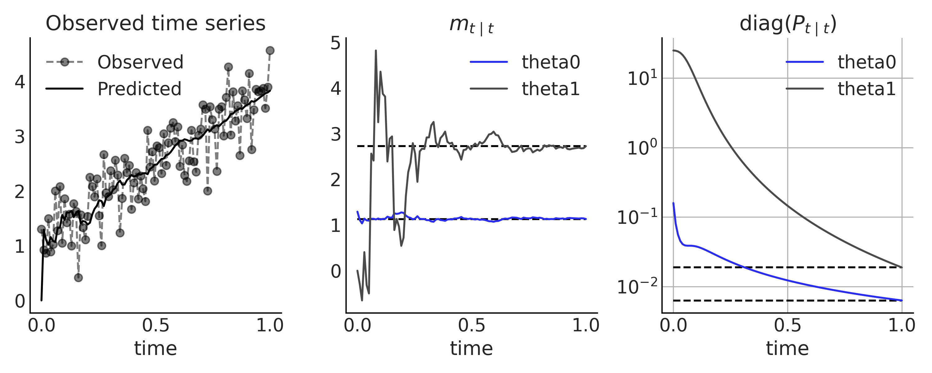
Fig. 6.16 Linear Growth time series model, inference using a Kalman filter. In the first panel we show the observed data (gray dot connected by dash line) and the one-step prediction from the Kalman filter (\(H_t m_{t \mid t-1}\) in solid black line). The posterior distribution of the latent state \(X_t\) after observing each time step is compared with the closed form solution using all data (black solid line) in the middle and rightmost panel.#
6.4.2. ARIMA, Expressed as a State Space Model#
State space models are a unified methodology that generalized many classical time series models. However, it might not always be obvious how we can express a model in state space format. In this section we will look at how to express a more complex linear Gaussian state space model: ARMA and ARIMA. Recall the ARMA(p,q) Equation (6.8) from above, we have the AR coefficient parameters \(\phi_i\), the MA coefficient \(\theta_j\), and noise parameter \(\sigma\). It is tempting to use \(\sigma\) to parameterize the observation noise distribution \(R_t\). However, the moving average of the noise from the previous steps in the ARMA(p,q) Equation (6.8) requires us to “record” the current noise. The only solution is to formulate it into the transition noise so it becomes part of the latent state \(X_t\). First, we reformulate ARMA(p,q) Equation (6.8) into:
where the constant term \(\alpha\) from Equation (6.8) is omitted, and \(r = max(p, q+1)\). We pad zeros to coefficient parameters \(\phi\) and \(\theta\) when needed so that they have the same size \(r\). The component of the state equation for \(X_t\) is thus:
With the latent state being:
The observation operator is thus simply an indexing matrix \(\mathbf{H}_t = [1, 0, 0, \dots, 0]\) with the observation equation being \(y_t = \mathbf{H}_t X_t\) [14].
For example, an ARMA(2,1) model in state space representation is:
You might notice that the state transition is slightly different than what we defined above, as the transition noise is not drawn from a Multivariate Gaussian distribution. The covariance matrix of \(\eta\) is \(\mathbf{Q}_t = \mathbf{A} \sigma^2 \mathbf{A}^T\), which in this case results in a singular random variable \(\eta\). Nonetheless, we can define the model in TFP. For example, in Code Block tfd_lgssm_arma_simulate we defines a ARMA(2,1) model with \(\phi = [-0.1, 0.5]\), \(\theta = -0.25\), and \(\sigma = 1.25\), and draw one random time series.
num_timesteps = 300
phi1 = -.1
phi2 = .5
theta1 = -.25
sigma = 1.25

# X_0
initial_state_prior = tfd.MultivariateNormalDiag(
   scale_diag=[sigma, sigma])
# F_t
transition_matrix = lambda _: tf.linalg.LinearOperatorFullMatrix(
   [[phi1, 1], [phi2, 0]])
# eta_t ~ Normal(0, Q_t)
R_t = tf.constant([[sigma], [sigma*theta1]])
Q_t_tril = tf.concat([R_t, tf.zeros_like(R_t)], axis=-1)
transition_noise = lambda _: tfd.MultivariateNormalTriL(
   scale_tril=Q_t_tril)
# H_t
observation_matrix = lambda t: tf.linalg.LinearOperatorFullMatrix(
   [[1., 0.]])
# epsilon_t ~ Normal(0, 0)
observation_noise = lambda _: tfd.MultivariateNormalDiag(
   loc=[0.], scale_diag=[0.])

arma = tfd.LinearGaussianStateSpaceModel(
   num_timesteps=num_timesteps,
   transition_matrix=transition_matrix,
   transition_noise=transition_noise,
   observation_matrix=observation_matrix,
   observation_noise=observation_noise,
   initial_state_prior=initial_state_prior
   )

sim_ts = arma.sample()  # Simulate from the model
Adding the appropriate prior and some small rewrite to handle the shape
a bit better, we can get a full generative ARMA(2,1) model in Code Block
tfd_lgssm_arma_with_prior.
Conditioning on the (simulated) data sim_ts and running inference are
straightforward since we are working with a
tfd.JointDistributionCoroutine model. Note that the unknown parameters
are not part of the latent state \(X_t\), thus instead of a Bayesian
filter like Kalman filter, inference is done using standard MCMC method.
We show the resulting trace plot of the posterior samples in
Fig. 6.17.
@tfd.JointDistributionCoroutine
def arma_lgssm():
    sigma = yield root(tfd.HalfStudentT(df=7, loc=0, scale=1., name="sigma"))
    phi = yield root(tfd.Sample(tfd.Normal(0, 0.5), 2, name="phi"))
    theta = yield root(tfd.Sample(tfd.Normal(0, 0.5), 1, name="theta"))
    # Prior for initial state
    init_scale_diag = tf.concat([sigma[..., None], sigma[..., None]], axis=-1)
    initial_state_prior = tfd.MultivariateNormalDiag(
        scale_diag=init_scale_diag)

    F_t = tf.concat([phi[..., None],
                     tf.concat([tf.ones_like(phi[..., 0, None]),
                                tf.zeros_like(phi[..., 0, None])],
                               axis=-1)[..., None]],
                    axis=-1)
    transition_matrix = lambda _: tf.linalg.LinearOperatorFullMatrix(F_t)

    transition_scale_tril = tf.concat(
        [sigma[..., None], theta * sigma[..., None]], axis=-1)[..., None]
    scale_tril = tf.concat(
        [transition_scale_tril,
         tf.zeros_like(transition_scale_tril)],
        axis=-1)
    transition_noise = lambda _: tfd.MultivariateNormalTriL(
        scale_tril=scale_tril)

    observation_matrix = lambda t: tf.linalg.LinearOperatorFullMatrix([[1., 0.]])
    observation_noise = lambda t: tfd.MultivariateNormalDiag(
        loc=[0], scale_diag=[0.])

    arma = yield tfd.LinearGaussianStateSpaceModel(
            num_timesteps=num_timesteps,
            transition_matrix=transition_matrix,
            transition_noise=transition_noise,
            observation_matrix=observation_matrix,
            observation_noise=observation_noise,
            initial_state_prior=initial_state_prior,
            name="arma")

Fig. 6.17 MCMC sampling result from the ARMA(2,1) model arma_lgssm defined in
Code Block
tfd_lgssm_arma_with_prior,
conditioned on the simulated data sim_ts generated in Code Block
tfd_lgssm_arma_simulate. The
true values of the parameters are plotted as vertical lines in the
posterior density plot and horizontal lines in the trace plot.#
We can already use this formulation for ARIMA modeling with \(d>0\) by preprocessing the observed time series to account for the integrated part. However, state space model representation gives us an advantage where we can write down the generative process directly and more intuitively without taking the repeated differences \(d\) times on the observation in the data preprocessing step.
For example, consider extending the ARMA(2,1) model above with \(d=1\), we have \(\Delta y_t = y_t - y_{t-1}\), which means \(y_t = y_{t-1} + \Delta y_t\) and we can define observation operator as \(\mathbf{H}_t = [1, 1, 0]\), with the latent state \(X_t\) and state transition being:
As you can see, while the parameterization results in a larger size latent state vector \(X_t\), the number of parameters stays the same. Moreover, the model is generative in \(y_t\) instead of \(\Delta y_t\). However, challenges may arise when specifying the distribution of the initial state \(X_0\), as the first elements (\(y_0\)) are now non-stationary. In practice, we can assign an informative prior around the initial value of the time series after centering (subtracting the mean). More discussion around this topic and an in depth introduction to state space models for time series problems could be found in Durbin and Koopman [61].
6.4.3. Bayesian Structural Time Series#
A linear Gaussian state space representation of a time series model has another advantage that it is easily extendable, especially with other linear Gaussian state space models. To combine two models, we follow the same idea of concatenating two normal random variables in the latent space. We generate a block diagonal matrix using the 2 covariance matrix, concatenating the mean on the event axis. In the measurement space the operation is equivalent to summing two normal random variables. More concretely, we have:
If we have a time series model \(\mathcal{M}\) that is not linear Gaussian. We can also incorporate it into a state space model. To do that, we treat the prediction \(\hat{\psi}_t\) from \(\mathcal{M}\) at each time step as a static “known” value and add to the observation noise distribution \(\epsilon_t \sim N(\hat{\mu}_t + \hat{\psi}_t, R_t)\). Conceptually we can understand it as subtracting the prediction of \(\mathcal{M}\) from \(Y_t\) and modeling the result, so that the Kalman filter and other linear Gaussian state space model properties still hold.
This composability feature makes it easy to build a time series model
that is constructed from multiple smaller linear Gaussian state space
model components. We can have individual state space representations for
the trend, seasonal, and error terms, and combine them into what is
usually referred to as a structural time series model or dynamic
linear model. TFP provides a very convenient way to build Bayesian
structural time series with the tfp.sts module, along with helper
functions to deconstruct the components, make forecasts, inference, and
other diagnostics.
For example, we can model the monthly birth data using a structural time series with a local linear trend component and a seasonal component to account for the monthly pattern in Code Block tfp_sts_example2.
def generate_bsts_model(observed=None):
    """
    Args:
        observed: Observed time series, tfp.sts use it to generate prior.
    """
    # Trend
    trend = tfp.sts.LocalLinearTrend(observed_time_series=observed)
    # Seasonal
    seasonal = tfp.sts.Seasonal(num_seasons=12, observed_time_series=observed)
    # Full model
    return tfp.sts.Sum([trend, seasonal], observed_time_series=observed)

observed = tf.constant(us_monthly_birth["birth_in_thousands"], dtype=tf.float32)
birth_model = generate_bsts_model(observed=observed)

# Generate the posterior distribution conditioned on the observed
target_log_prob_fn = birth_model.joint_log_prob(observed_time_series=observed)
We can inspect each component in birth_model:
birth_model.components
[<tensorflow_probability.python.sts.local_linear_trend.LocalLinearTrend at ...>,
 <tensorflow_probability.python.sts.seasonal.Seasonal at ...>]
Each of the components is parameterized by some hyperparameters, which are the unknown parameters that we want to do inference on. They are not part of the latent state \(X_t\), but might parameterize the prior that generates \(X_t\). For example, we can check the parameters of the seasonal component:
birth_model.components[1].parameters
[Parameter(name='drift_scale', prior=<tfp.distributions.LogNormal
'Seasonal_LogNormal' batch_shape=[] event_shape=[] dtype=float32>,
bijector=<tensorflow_probability.python.bijectors.chain.Chain object at ...>)]
Here the seasonal component of the STS model contains 12 latent states (one for each month), but the component only contains 1 parameter (the hyperparameter that parameterized the latent states). You might have already noticed from examples in the previous session how unknown parameters are treated differently. In the linear growth model, unknown parameters are part of the latent state \(X_t\), in the ARIMA model, the unknown parameters parameterized \(\mathbf{F}_t\) and \(\mathbf{Q}_t\). For the latter case, we cannot use Kalman filter to infer those parameters. Instead, the latent state is effectively marginalized out but we can nonetheless recover them after inference by running the Kalman filter conditioned on the posterior distribution (represented as Monte Carlo Samples). A conceptual description of the parameterization could be found in the Fig. 6.18:
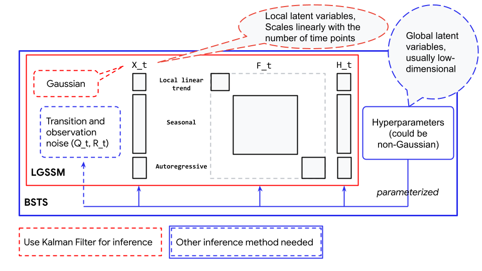
Fig. 6.18 Relationship between Bayesian Structural Time Series (blue box) and Linear Gaussian State Space Model (red box). The Linear Gaussian State Space Model shown here is an example containing a local linear trend component, a seasonal component, and an Autoregressive component.#
Thus running inference on a structural time series model could conceptually be understood as generating a linear Gaussian state space model from the parameters to be inferred, running the Kalman filter to obtain the data likelihood, and combining with the prior log-likelihood conditioned on the current value of the parameters. Unfortunately, the operation of iterating through each data point is quite computationally costly (even though Kalman filter is already an extremely efficient algorithm), thus fitting structural time series may not scale very well when running long time series.
After running inference on a structural time series model there are some
helpful utility functions from tfp.sts we can use to make forecast and
inspect each inferred component with Code Block
tfp_sts_example2_result. The
result is shown in Fig. 6.19.
# Using a subset of posterior samples.
parameter_samples = [x[-100:, 0, ...] for x in mcmc_samples]

# Get structual compoenent.
component_dists = tfp.sts.decompose_by_component(
    birth_model,
    observed_time_series=observed,
    parameter_samples=parameter_samples)

# Get forecast for n_steps.
n_steps = 36
forecast_dist = tfp.sts.forecast(
    birth_model,
    observed_time_series=observed,
    parameter_samples=parameter_samples,
    num_steps_forecast=n_steps)
birth_dates = us_monthly_birth.index
forecast_date = pd.date_range(
    start=birth_dates[-1] + np.timedelta64(1, "M"),
    end=birth_dates[-1] + np.timedelta64(1 + n_steps, "M"),
    freq="M")

fig, axes = plt.subplots(
    1 + len(component_dists.keys()), 1, figsize=(10, 9), sharex=True)

ax = axes[0]
ax.plot(us_monthly_birth, lw=1.5, label="observed")

forecast_mean = np.squeeze(forecast_dist.mean())
line = ax.plot(forecast_date, forecast_mean, lw=1.5,
               label="forecast mean", color="C4")

forecast_std = np.squeeze(forecast_dist.stddev())
ax.fill_between(forecast_date,
                forecast_mean - 2 * forecast_std,
                forecast_mean + 2 * forecast_std,
                color=line[0].get_color(), alpha=0.2)

for ax_, (key, dist) in zip(axes[1:], component_dists.items()):
    comp_mean, comp_std = np.squeeze(dist.mean()), np.squeeze(dist.stddev())
    line = ax_.plot(birth_dates, dist.mean(), lw=2.)
    ax_.fill_between(birth_dates,
                     comp_mean - 2 * comp_std,
                     comp_mean + 2 * comp_std,
                     alpha=0.2)
    ax_.set_title(key.name[:-1])
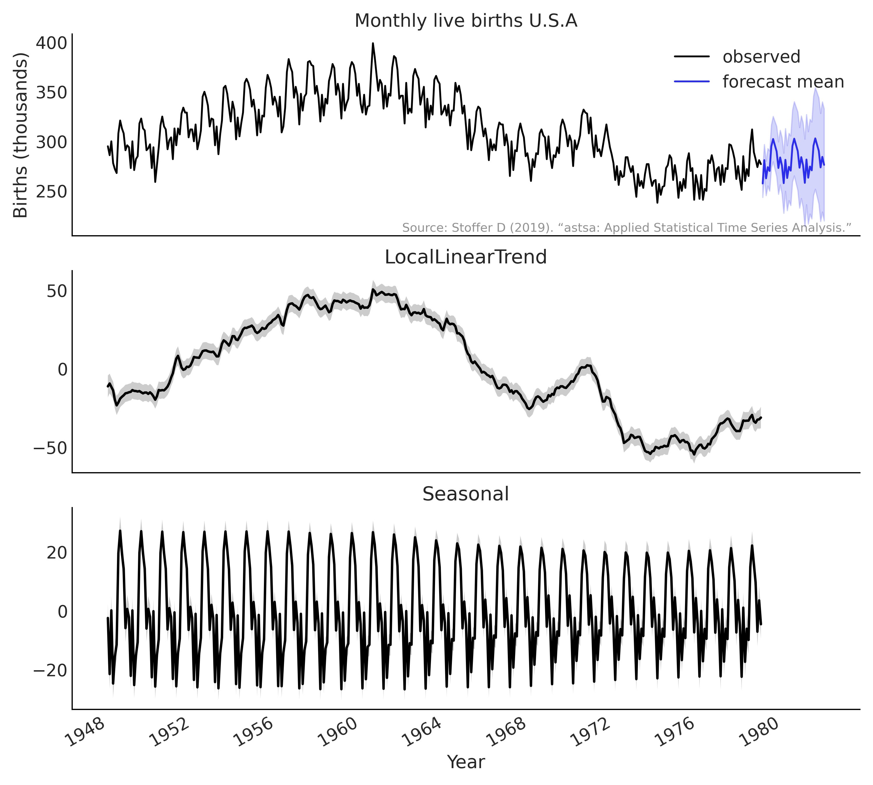
Fig. 6.19 Inference result and forecast of monthly live births in the United
States (1948-1979) using the tfp.sts API with Code Block
tfp_sts_example2_result. Top
panel: 36 months forecast; bottom 2 panels: decomposition of the
structural time series.#
6.5. Other Time Series Models#
While structural time series and linear Gaussian state space models are powerful and expressive classes of time series models, they certainly do not cover all our needs. For example, some interesting extensions include nonlinear Gaussian state space models, where the transition function and measurement function are differentiable nonlinear functions. Extended Kalman filter could be used for inference of \(X_t\) for these models [62]. There is the Unscented Kalman filter for inference of non-Gaussian nonlinear models [62], and Particle filter as a general filtering approach for state space models [63].
Another class of widely used time series models is the Hidden Markov model, which is a state space model with discrete state space. There are also specialized algorithms for doing inference of these models, for example, the forward-backward algorithm for computing the marginal posterior likelihood, and the Viterbi algorithm for computing the posterior mode.
In addition there are ordinary differential equations (ODE) and stochastic differential equations (SDE) that are continuous time models. In Table 6.2 we divide the space of models by their treatment of stochasticity and time. While we are not going into details of these models, they are well studied subjects with easy to use implementations in the Python computing ecosystem.
Deterministic dynamics |
Stochastic dynamics |
|
Discrete time |
automata / discretized ODEs |
state space models |
Continuous time |
ODEs |
SDEs |
6.6. Model Criticism and Choosing Priors#
In the seminal time series book by Box et al. [57] [15], they outlined five important practical problems for time series modeling:
Forecasting
Estimation of Transfer Functions
Analysis of Effects of Unusual Intervention Events to a System
Analysis of Multivariate Time Series
Discrete Control Systems
In practice, most time series problems aim at performing some sort of forecasting (or nowcasting where you try to infer at instantaneous time \(t\) some observed quantity that are not yet available due to delay in getting the measurements), which sets up a natural model criticism criteria in time series analysis problems. While we do not have specific treatment around Bayesian decision theory in this chapter, It is worth quoting from West and Harrison [59]:
Good modeling demands hard thinking, and good forecasting requires an integrated view of the role of forecasting within decision systems.
In practice, criticism of time series model inference and evaluation of forecasting should be closely integrated with the decision making process, especially how uncertainty should be incorporated into decisions. Nonetheless, forecast performance could be evaluated alone. Usually this is done by collecting new data or keeping some hold out dataset as we did in this Chapter for the CO₂ example, and compare the observation with the forecast using standard metrics. One of a popular choice is Mean Absolute Percentage Error (MAPE), which simply compute:
However, there are some known biases of MAPE, for example, large errors during low value observation periods will significantly impact MAPE. Also, it is difficult to compare MAPE across multiple time series when the range of observation differs greatly.
Cross-validation based model evaluation approaches still apply and are recommended for time series models. However, using LOO for a single time series will be problematic if the goal is to estimate the predictive performance for future time points. Simply leaving out one observation at a time does not respect the temporal structure of the data (or model). For example, if you remove one point \(t\) and use the rest of the points for predictions you will be using the points \(t_{-1}, t_{-2}, ...\) which may be fine as previous observations (up to some point) inform future ones, but you will be also using points \(t_{+1}, t_{+2}, ...\), that is you will be using the future to predict the past. Thus, we can compute LOO, but the interpretation of the number will get will be nonsensical and thus misleading. Instead of leaving one (or some) time points out, we need some form of leave-future-out cross-validation (LFO-CV, see e.g. Bürkner et al. [64]. As a rough sketch, after initial model inference, to approximate 1-step-ahead predictions we would iterate over the hold out time series or future observations and evaluate on the log predictive density, and refit the model including a specific time point when the Pareto \(k\) estimate exceeds some threshold [16]. Thus, LFO-CV does not refer to one particular prediction task but rather to various possible cross validation approaches that all involve some form of prediction of future time points.
6.6.1. Priors for Time Series Models#
In Section Basis Functions and Generalized Additive Model we used a regularizing prior, the Laplace prior, for the slope of the step linear function. As we mentioned this is to express our prior knowledge that the change in slope is usually small and close to zero, so that the resulting latent trend is smoother. Another common use of regularizing priors or sparse priors, is for modeling holiday or special days effect. Usually each holiday has its own coefficients, and we want to express a prior that indicates some holidays could have huge effect on the time series, but most holidays are just like any other ordinary day. We can formalize this intuition with a horseshoe prior [65, 66] as shown in Equation (6.25):
The global parameter \(\tau\) in the horseshoe prior pulls the coefficients of the holiday effect globally towards zero. Meanwhile, the heavy tail from the local scales \(\lambda_t\) let some effect break out from the shrinkage. We can accommodate different levels of sparsity by changing the value of \(\tau\): the closer \(\tau\) is to zero the more shrinkage of the holiday effect \(\beta_t\) to tends to zero, whereas with a larger \(\tau\) we have a more diffuse prior [67] [17]. For example, in Case Study 2 of Riutort-Mayol et al. [68] they included a special day effect for each individual day of a year (366 as the Leap Day is included) and use a horseshoe prior to regularize it.
Another important consideration of prior for time series model is the prior for the observation noise. Most time series data are by nature are non-repeated measures. We simply cannot go back in time and make another observation under the exact condition (i.e., we cannot quantify the aleatoric uncertainty). This means our model needs information from the prior to “decide” whether the noise is from measurement or from latent process (i.e., the epistemic uncertainty). For example, in a time series model with a latent autoregressive component or a local linear trend model, we can place more informative prior on the observation noise to regulate it towards a smaller value. This will “push” the trend or autoregressive component to overfits the underlying drift pattern and we might have a nicer forecast on the trend (higher forecast accuracy in the short term). The risk is that we are overconfident about the underlying trend, which will likely result in a poor forecast in the long run. In a real world application where time series are most likely non-stationary, we should be ready to adjust the prior accordingly.
6.7. Exercises#
6E1. As we explained in Box Parsing timestamp to design matrix above, date information could be formatted into a design matrix for regression model to account for the periodic pattern in a time series. Try generating the following design matrix for the year 2021. Hint: use Code Block timerange_2021 to generate all time stamps for 2021:
datetime_index = pd.date_range(start="2021-01-01", end="2021-12-31", freq='D')
A design matrix for day of the month effect.
A design matrix for weekday vs weekend effect.
Company G pay their employee on the 25th of every month, and if the 25th falls on a weekend, the payday is moved up to the Friday before. Try to create a design matrix to encode the pay day of 2021.
A design matrix for the US Federal holiday effect [18] in 2021. Create the design matrix so that each holiday has their individual coefficient.
6E2. In the previous exercise , the design matrix for holiday effect treat each holiday separately. What if we consider all holiday effects to be the same? What is the shape of the design matrix if we do so? Reason about how does it affects the fit of the regression time series model.
6E3. Fit a linear regression to the
"monthly_mauna_loa_co2.csv" dataset:
A plain regression with an intercept and slope, using linear time as predictor.
A covariate adjusted regression like the square root predictor in the baby example in Chapter 4 Code Block babies_transformed.
Explain what these models are missing compared to Code Block regression_model_for_timeseries.
6E4. Explain in your own words the difference between regression, autoregressive and state space architectures. In which situation would each be particularly useful.
6M5. Does using basis function as design matrix actually
have better condition number than sparse matrix? Compare the condition
number of the following design matrix of the same rank using
numpy.linalg.cond:
Dummy coded design matrix
seasonality_allfrom Code Block generate_design_matrix.Fourier basis function design matrix
X_predfrom Code Block gam.An array of the same shape as
seasonality_allwith values drawn from a Normal distribution.An array of the same shape as
seasonality_allwith values drawn from a Normal distribution and one of the column being identical to another.
6M6. The gen_fourier_basis function from Code Block
fourier_basis_as_seasonality
takes a time index t as the first input. There are a few different
ways to represent the time index, for example, if we are observing some
data monthly from 2019 January for 36 months, we can code the time index
in 2 equivalent ways as shown below in Code Block
exercise_chap4_e6:
nmonths = 36
day0 = pd.Timestamp('2019-01-01')
time_index = pd.date_range(
    start=day0, end=day0 + np.timedelta64(nmonths, 'M'),
    freq='M')

t0 = np.arange(len(time_index))
design_matrix0 = gen_fourier_basis(t0, p=12, n=6)
t1 = time_index.month - 1
design_matrix1 = gen_fourier_basis(t1, p=12, n=6)

np.testing.assert_array_almost_equal(design_matrix0, design_matrix1)
What if we are observing the data daily? How would you change the Code Block exercise_chap4_e6 to:
Make
time_indexrepresent day of the year instead of month of the year.Modify the function signature to
gen_fourier_basisin line 8 and 10 so that the resulting design matrices coded for the month of the year effect.How does the new
design_matrix0anddesign_matrix1differ? How is the differences would impact the model fitting? Hint: validate your reasoning by multiplying them with the same random regression coefficient.
6E7. In Section Autoregressive Models we introduced the backshift operator \(\mathbf{B}\). You might have already noticed that applying the operation \(\mathbf{B}\) on a time series is the same as performing a matrix multiplication. We can generate a matrix \(\mathbf{B}\) explicitly in Python. Modify Code Block ar1_without_forloop to use an explicit \(\mathbf{B}\) constructed in NumPy or TensorFlow.
6E8. The step linear function as defined in Equation (6.3) and Code Block step_linear_function_for_trend rely on a key regression coefficient \(\delta\). Rewrite the definition so that it has a similar form compare to other linear regression:
Find the appropriate expression of design matrix \(\mathbf{A}^\prime\) and coefficient \(\delta^\prime\).
6E9. As we have seen in past chapters, a great way to
understand your data generating process is to write it down. In this
exercise we will generate synthetic data which will reinforce the
mapping of “real world” ideas to code. Assume we start with a linear
trend that is y = 2x, x = np.arange(90), and iid noise at each time
point draw from a \(\mathcal{N}(0, 1)\). Assume that this time series
starts on Sunday June 6 2021. Generate 4 synthetic datasets that
include:
An additive weekend effect where weekends have 2x more volume than weekdays.
An additive sinusoidal effect of sin(2x).
An additive AR(1) latent process with autoregressive coefficient of your choice and a noise scale \(\sigma = 0.2\).
A time series with weekend and sinusoidal effect from (1) and (2), and an AR(1) process on the mean of the time series with the same autoregressive coefficient as in (3)
6E10. Adapt the model in Code Block gam_with_ar_likelihood to model the generated time series in 6E9 (4).
6E11. Inspection of the inference result (MCMC trace and
diagnostic) of models in this chapter using ArviZ. For example, look
at:
Trace plot
Rank plot
Summary of posterior sample
Which model contains problematic chains (divergence, low ESS, large \(\hat R\))? Could you find ways to improve the inference for those models?
6M12. Generate a sinusoidal time series with 200 time
points in Python, and fit it with a AR(2) model. Do that in TFP by
modifying Code Block
ar1_without_forloop and in PyMC3
with pm.AR API.
6M13. This is an exercise of posterior predictive check for AR models. Generate the prediction distribution at each time step \(t\) for the AR2 model in Exercise 6M11. Note that for each time step \(t\) you need to condition on all the observations up to time step \(t-1\). Does the one-step-ahead predictive distribution match the observed time series?
6M14. Make forecast for 50 time steps using the AR2 models from Exercise 6M11. Does the forecast also look like a sinusoidal signal?
6H15. Implement the generative process for the \(\text{SARIMA}(1, 1, 1)(1, 1, 1)_{12}\) model, and make forecast.
6M16. Implement and inference a \(ARIMAX(1,1,1)X[4]\) model for the monthly birth dataset in this chapter, with the design matrix generated from a Fourier basis functions with \(N=2\).
6H17. Derive the Kalman filter equations. Hint: first work out the joint distribution of \(X_t\) and \(X_{t-1}\), and then follow with the joint distribution of \(Y_t\) and \(X_t\). If you are still stuck take at look at Chapter 4 in Särkkä’s book [60].
6M18. Inspect the output of
linear_growth_model.forward_filter by indexing to a given time step:
Identify the input and output of one Kalman filter step;
Compute one step of the Kalman filter predict and update step using the input;
Assert that your computation is the same as the indexed output.
6M19. Study the documentation and implementation of
tfp.sts.Seasonal, and answer the following questions:
How many hyperparameters does a seasonal SSM contains?
How does it parameterized the latent states and what kind of regularization effect does the prior has? Hint: draw connection to the Gaussian Random Walk prior in Chapter 5.
6M20. Study the documentation and implementation of
tfp.sts.LinearRegression and tfp.sts.Seasonal, and reason about the
differences of SSM they represent when modeling a day of the week
pattern:
How is the day of the week coefficient represented? Are they part of the latent states?
How is the model fit different between the two SSMs? Validate your reasoning with simulations.